Stellarium 26.3 User Guide
Georg Zotti, Alexander Wolf (editors)
2026

Copyright © 2014-2026 Georg Zotti.
Copyright © 2011-2026 Alexander Wolf.
Copyright © 2006-2013 Matthew Gates.
Copyright © 2013-2014 Barry Gerdes († 2014).
STELLARIUM.ORG
Permission is granted to copy, distribute and/or modify this document under the terms of the GNU
Free Documentation License, Version 1.3 or any later version published by the Free Software
Foundation; with no Invariant Sections, no Front-Cover Texts, and no Back-Cover Texts. A copy of
the license is included in the appendix G entitled “GNU Free Documentation License”.
All trademarks, third party brands, product names, trade names, corporate names and company names
mentioned may be trademarks of their respective owners or registered trademarks of other companies and
are used for purposes of explanation and to the readers’ benefit, without implying a violation of copyright law.
Version 26.3-1, September 28, 2026
Contents
I
Basic Use
1 Introduction . . . . . . . . . . . . . . . . . . . . . . . . . . . . . . . . . . . . . . . . . . . . . . . . . . . 3
1.1 Historical notes . . . . . . . . . . . . . . . . . . . . . . . . . . . . . . . . . . . . . . . . . . . . . . . . . . 3
1.2 Version Numbers . . . . . . . . . . . . . . . . . . . . . . . . . . . . . . . . . . . . . . . . . . . . . . . . . 5
1.3 Acknowledgements . . . . . . . . . . . . . . . . . . . . . . . . . . . . . . . . . . . . . . . . . . . . . . 5
1.4 Scientific use . . . . . . . . . . . . . . . . . . . . . . . . . . . . . . . . . . . . . . . . . . . . . . . . . . . . 5
1.5 About this User Guide . . . . . . . . . . . . . . . . . . . . . . . . . . . . . . . . . . . . . . . . . . . . . 6
2 Getting Started . . . . . . . . . . . . . . . . . . . . . . . . . . . . . . . . . . . . . . . . . . . . . . . . 7
2.1 System Requirements . . . . . . . . . . . . . . . . . . . . . . . . . . . . . . . . . . . . . . . . . . . . . . 7
2.1.1 Minimum . . . . . . . . . . . . . . . . . . . . . . . . . . . . . . . . . . . . . . . . . . . . . . . . . . . . . . . 7
2.1.2 Recommended . . . . . . . . . . . . . . . . . . . . . . . . . . . . . . . . . . . . . . . . . . . . . . . . . . 7
2.2 Downloading . . . . . . . . . . . . . . . . . . . . . . . . . . . . . . . . . . . . . . . . . . . . . . . . . . . . 8
2.3 Installation . . . . . . . . . . . . . . . . . . . . . . . . . . . . . . . . . . . . . . . . . . . . . . . . . . . . . . 8
2.3.1 Windows . . . . . . . . . . . . . . . . . . . . . . . . . . . . . . . . . . . . . . . . . . . . . . . . . . . . . . . 8
2.3.2 macOS . . . . . . . . . . . . . . . . . . . . . . . . . . . . . . . . . . . . . . . . . . . . . . . . . . . . . . . . . 8
2.3.3 Linux . . . . . . . . . . . . . . . . . . . . . . . . . . . . . . . . . . . . . . . . . . . . . . . . . . . . . . . . . . . 8
2.3.4 *BSD/Solaris/OpenIndiana . . . . . . . . . . . . . . . . . . . . . . . . . . . . . . . . . . . . . . . . . . 9
2.3.5 Haiku . . . . . . . . . . . . . . . . . . . . . . . . . . . . . . . . . . . . . . . . . . . . . . . . . . . . . . . . . . 9
2.4 Running Stellarium . . . . . . . . . . . . . . . . . . . . . . . . . . . . . . . . . . . . . . . . . . . . . . . . 9
2.4.1 Windows . . . . . . . . . . . . . . . . . . . . . . . . . . . . . . . . . . . . . . . . . . . . . . . . . . . . . . . 9
2.4.2 macOS . . . . . . . . . . . . . . . . . . . . . . . . . . . . . . . . . . . . . . . . . . . . . . . . . . . . . . . . . 9
2.4.3 Linux . . . . . . . . . . . . . . . . . . . . . . . . . . . . . . . . . . . . . . . . . . . . . . . . . . . . . . . . . . . 9
2.4.4 *BSD/Solaris/OpenIndiana . . . . . . . . . . . . . . . . . . . . . . . . . . . . . . . . . . . . . . . . . . 9
2.4.5 Haiku . . . . . . . . . . . . . . . . . . . . . . . . . . . . . . . . . . . . . . . . . . . . . . . . . . . . . . . . . . 9
2.5 Script Launch . . . . . . . . . . . . . . . . . . . . . . . . . . . . . . . . . . . . . . . . . . . . . . . . . . . 10
2.6 Troubleshooting . . . . . . . . . . . . . . . . . . . . . . . . . . . . . . . . . . . . . . . . . . . . . . . . . 10

3 A First Tour . . . . . . . . . . . . . . . . . . . . . . . . . . . . . . . . . . . . . . . . . . . . . . . . . . . 11
3.1 Time Travel . . . . . . . . . . . . . . . . . . . . . . . . . . . . . . . . . . . . . . . . . . . . . . . . . . . . . 12
3.2 Moving Around the Sky . . . . . . . . . . . . . . . . . . . . . . . . . . . . . . . . . . . . . . . . . . . 13
3.3 The Main Tool Bar . . . . . . . . . . . . . . . . . . . . . . . . . . . . . . . . . . . . . . . . . . . . . . . . 14
3.4 Exporting data . . . . . . . . . . . . . . . . . . . . . . . . . . . . . . . . . . . . . . . . . . . . . . . . . . 16
3.4.1 Taking Screenshots . . . . . . . . . . . . . . . . . . . . . . . . . . . . . . . . . . . . . . . . . . . . . . . 16
3.4.2 Copy Information . . . . . . . . . . . . . . . . . . . . . . . . . . . . . . . . . . . . . . . . . . . . . . . . 16
3.4.3 Scripting . . . . . . . . . . . . . . . . . . . . . . . . . . . . . . . . . . . . . . . . . . . . . . . . . . . . . . . 16
3.5 Observing Lists (Bookmarks) . . . . . . . . . . . . . . . . . . . . . . . . . . . . . . . . . . . . . . . 17
3.6 Custom Markers . . . . . . . . . . . . . . . . . . . . . . . . . . . . . . . . . . . . . . . . . . . . . . . . . 17
3.7 Speech Output . . . . . . . . . . . . . . . . . . . . . . . . . . . . . . . . . . . . . . . . . . . . . . . . . . 17
4 The User Interface . . . . . . . . . . . . . . . . . . . . . . . . . . . . . . . . . . . . . . . . . . . . 19
4.1 Setting the Date and Time . . . . . . . . . . . . . . . . . . . . . . . . . . . . . . . . . . . . . . . . . 19
4.2 Setting Your Location . . . . . . . . . . . . . . . . . . . . . . . . . . . . . . . . . . . . . . . . . . . . . 20
4.2.1 Time Zones . . . . . . . . . . . . . . . . . . . . . . . . . . . . . . . . . . . . . . . . . . . . . . . . . . . . . 21
4.2.2 Geographical Regions . . . . . . . . . . . . . . . . . . . . . . . . . . . . . . . . . . . . . . . . . . . 21
4.2.3 Observers . . . . . . . . . . . . . . . . . . . . . . . . . . . . . . . . . . . . . . . . . . . . . . . . . . . . . . 21
4.3 The Configuration Window . . . . . . . . . . . . . . . . . . . . . . . . . . . . . . . . . . . . . . . . . 21
4.3.1 The Main Tab . . . . . . . . . . . . . . . . . . . . . . . . . . . . . . . . . . . . . . . . . . . . . . . . . . . 21
4.3.2 The Information Tab . . . . . . . . . . . . . . . . . . . . . . . . . . . . . . . . . . . . . . . . . . . . . . 22
4.3.3 The Extras Tab . . . . . . . . . . . . . . . . . . . . . . . . . . . . . . . . . . . . . . . . . . . . . . . . . . . 23
4.3.4 The Time Tab . . . . . . . . . . . . . . . . . . . . . . . . . . . . . . . . . . . . . . . . . . . . . . . . . . . 24
4.3.5 The Tools Tab . . . . . . . . . . . . . . . . . . . . . . . . . . . . . . . . . . . . . . . . . . . . . . . . . . . 24
4.3.6 The Speech Tab . . . . . . . . . . . . . . . . . . . . . . . . . . . . . . . . . . . . . . . . . . . . . . . . . 26
4.3.7 The Scripts Tab . . . . . . . . . . . . . . . . . . . . . . . . . . . . . . . . . . . . . . . . . . . . . . . . . . 27
4.3.8 The Plugins Tab . . . . . . . . . . . . . . . . . . . . . . . . . . . . . . . . . . . . . . . . . . . . . . . . . . 27
4.4 The View Settings Window . . . . . . . . . . . . . . . . . . . . . . . . . . . . . . . . . . . . . . . . . 27
4.4.1 The Sky Tab . . . . . . . . . . . . . . . . . . . . . . . . . . . . . . . . . . . . . . . . . . . . . . . . . . . . 29
4.4.2 The Solar System Objects (SSO) Tab . . . . . . . . . . . . . . . . . . . . . . . . . . . . . . . . . . 31
4.4.3 The Deep-Sky Objects (DSO) Tab . . . . . . . . . . . . . . . . . . . . . . . . . . . . . . . . . . . 32
4.4.4 The Markings Tab . . . . . . . . . . . . . . . . . . . . . . . . . . . . . . . . . . . . . . . . . . . . . . . . 32
4.4.5 The Landscape Tab . . . . . . . . . . . . . . . . . . . . . . . . . . . . . . . . . . . . . . . . . . . . . . 32
4.4.6 The Sky Culture Tab . . . . . . . . . . . . . . . . . . . . . . . . . . . . . . . . . . . . . . . . . . . . . . 34
4.4.7 The Surveys Tab . . . . . . . . . . . . . . . . . . . . . . . . . . . . . . . . . . . . . . . . . . . . . . . . . 37
4.5 The Search Window . . . . . . . . . . . . . . . . . . . . . . . . . . . . . . . . . . . . . . . . . . . . . . 37
4.5.1 The Object tab . . . . . . . . . . . . . . . . . . . . . . . . . . . . . . . . . . . . . . . . . . . . . . . . . 37
4.5.2 The SIMBAD tab . . . . . . . . . . . . . . . . . . . . . . . . . . . . . . . . . . . . . . . . . . . . . . . . . 40
4.5.3 The Position tab . . . . . . . . . . . . . . . . . . . . . . . . . . . . . . . . . . . . . . . . . . . . . . . . . 40
4.5.4 The Lists tab . . . . . . . . . . . . . . . . . . . . . . . . . . . . . . . . . . . . . . . . . . . . . . . . . . . . 40
4.5.5 The Options tab . . . . . . . . . . . . . . . . . . . . . . . . . . . . . . . . . . . . . . . . . . . . . . . . . 40
4.6 The Astronomical Calculations Window . . . . . . . . . . . . . . . . . . . . . . . . . . . . . . 41
4.6.1 The Positions Tab . . . . . . . . . . . . . . . . . . . . . . . . . . . . . . . . . . . . . . . . . . . . . . . . 41
4.6.2 The Ephemeris Tab . . . . . . . . . . . . . . . . . . . . . . . . . . . . . . . . . . . . . . . . . . . . . . . 42
4.6.3 The “Risings, Transits, and Settings” (RTS) Ta b . . . . . . . . . . . . . . . . . . . . . . . . . . . 42
4.6.4 The Phenomena Tab . . . . . . . . . . . . . . . . . . . . . . . . . . . . . . . . . . . . . . . . . . . . . 42
4.6.5 The Graphs Tab . . . . . . . . . . . . . . . . . . . . . . . . . . . . . . . . . . . . . . . . . . . . . . . . . 42
4.6.6 The “What’s Up Tonight” (WUT) Tab . . . . . . . . . . . . . . . . . . . . . . . . . . . . . . . . . . 48
4.6.7 The “Planetary Calculator” (PC) Tab . . . . . . . . . . . . . . . . . . . . . . . . . . . . . . . . . 51
4.6.8 The Eclipses Tab . . . . . . . . . . . . . . . . . . . . . . . . . . . . . . . . . . . . . . . . . . . . . . . . . 51

4.6.9 The Almanac Tab . . . . . . . . . . . . . . . . . . . . . . . . . . . . . . . . . . . . . . . . . . . . . . . . 54
4.7 The Help Window . . . . . . . . . . . . . . . . . . . . . . . . . . . . . . . . . . . . . . . . . . . . . . . . 55
4.7.1 The Help Tab . . . . . . . . . . . . . . . . . . . . . . . . . . . . . . . . . . . . . . . . . . . . . . . . . . . 55
4.7.2 The About Tab . . . . . . . . . . . . . . . . . . . . . . . . . . . . . . . . . . . . . . . . . . . . . . . . . . 55
4.7.3 The Log Tab . . . . . . . . . . . . . . . . . . . . . . . . . . . . . . . . . . . . . . . . . . . . . . . . . . . . 55
4.7.4 The Config Tab . . . . . . . . . . . . . . . . . . . . . . . . . . . . . . . . . . . . . . . . . . . . . . . . . . 55
4.8 Editing Keyboard Shortcuts . . . . . . . . . . . . . . . . . . . . . . . . . . . . . . . . . . . . . . . . 57
4.8.1 Example . . . . . . . . . . . . . . . . . . . . . . . . . . . . . . . . . . . . . . . . . . . . . . . . . . . . . . . 57
II
Advanced Use
5 Files and Directories . . . . . . . . . . . . . . . . . . . . . . . . . . . . . . . . . . . . . . . . . . 61
5.1 Directories . . . . . . . . . . . . . . . . . . . . . . . . . . . . . . . . . . . . . . . . . . . . . . . . . . . . . 61
5.1.1 Windows . . . . . . . . . . . . . . . . . . . . . . . . . . . . . . . . . . . . . . . . . . . . . . . . . . . . . . 61
5.1.2 macOS . . . . . . . . . . . . . . . . . . . . . . . . . . . . . . . . . . . . . . . . . . . . . . . . . . . . . . . . 62
5.1.3 Linux . . . . . . . . . . . . . . . . . . . . . . . . . . . . . . . . . . . . . . . . . . . . . . . . . . . . . . . . . . 62
5.1.4 *BSD/Solaris/OpenIndiana . . . . . . . . . . . . . . . . . . . . . . . . . . . . . . . . . . . . . . . . . 62
5.1.5 Haiku . . . . . . . . . . . . . . . . . . . . . . . . . . . . . . . . . . . . . . . . . . . . . . . . . . . . . . . . . 62
5.1.6 Customized Location . . . . . . . . . . . . . . . . . . . . . . . . . . . . . . . . . . . . . . . . . . . . . 62
5.2 Directory Structure . . . . . . . . . . . . . . . . . . . . . . . . . . . . . . . . . . . . . . . . . . . . . . . 62
5.3 The Logfile . . . . . . . . . . . . . . . . . . . . . . . . . . . . . . . . . . . . . . . . . . . . . . . . . . . . . 63
5.4 The Main Configuration File . . . . . . . . . . . . . . . . . . . . . . . . . . . . . . . . . . . . . . . . 63
5.5 Getting Extra Data . . . . . . . . . . . . . . . . . . . . . . . . . . . . . . . . . . . . . . . . . . . . . . . 63
5.5.1 More Stars . . . . . . . . . . . . . . . . . . . . . . . . . . . . . . . . . . . . . . . . . . . . . . . . . . . . . 63
5.5.2 More Deep-Sky Objects . . . . . . . . . . . . . . . . . . . . . . . . . . . . . . . . . . . . . . . . . . . 64
5.5.3 Alternative Planet Ephemerides: DE430, DE431, DE440, DE441 . . . . . . . . . . . . . 64
5.5.4 GPS Position . . . . . . . . . . . . . . . . . . . . . . . . . . . . . . . . . . . . . . . . . . . . . . . . . . . . 65
5.5.5 Modernized MESA3D libraries (Software OpenGL on Windows) . . . . . . . . . . . . 66
6 Advanced Options . . . . . . . . . . . . . . . . . . . . . . . . . . . . . . . . . . . . . . . . . . . 67
6.1 Command Line Options . . . . . . . . . . . . . . . . . . . . . . . . . . . . . . . . . . . . . . . . . . . 67
6.1.1 Examples . . . . . . . . . . . . . . . . . . . . . . . . . . . . . . . . . . . . . . . . . . . . . . . . . . . . . . 69
6.2 Environment Variables . . . . . . . . . . . . . . . . . . . . . . . . . . . . . . . . . . . . . . . . . . . . 69
6.2.1 Logfile tweaks . . . . . . . . . . . . . . . . . . . . . . . . . . . . . . . . . . . . . . . . . . . . . . . . . . 70
6.3 GUI Customizations . . . . . . . . . . . . . . . . . . . . . . . . . . . . . . . . . . . . . . . . . . . . . . 70
6.3.1 Panel transparency . . . . . . . . . . . . . . . . . . . . . . . . . . . . . . . . . . . . . . . . . . . . . . 70
6.3.2 Button brightness . . . . . . . . . . . . . . . . . . . . . . . . . . . . . . . . . . . . . . . . . . . . . . . . 70
6.3.3 Text shadow . . . . . . . . . . . . . . . . . . . . . . . . . . . . . . . . . . . . . . . . . . . . . . . . . . . . 71
6.3.4 User interface colors . . . . . . . . . . . . . . . . . . . . . . . . . . . . . . . . . . . . . . . . . . . . . 71
6.4 Spout . . . . . . . . . . . . . . . . . . . . . . . . . . . . . . . . . . . . . . . . . . . . . . . . . . . . . . . . . 71
6.5 Show effects . . . . . . . . . . . . . . . . . . . . . . . . . . . . . . . . . . . . . . . . . . . . . . . . . . . . 72
6.5.1 Sky Background . . . . . . . . . . . . . . . . . . . . . . . . . . . . . . . . . . . . . . . . . . . . . . . . . 72
6.5.2 Star Trails . . . . . . . . . . . . . . . . . . . . . . . . . . . . . . . . . . . . . . . . . . . . . . . . . . . . . . . 72
6.6 Spherical Mirror Mode for Planetarium Use . . . . . . . . . . . . . . . . . . . . . . . . . . . . 72
6.6.1 360° Projection . . . . . . . . . . . . . . . . . . . . . . . . . . . . . . . . . . . . . . . . . . . . . . . . . . 72
6.6.2 Projector Specifications . . . . . . . . . . . . . . . . . . . . . . . . . . . . . . . . . . . . . . . . . . . 73
6.6.3 Computer Configuration . . . . . . . . . . . . . . . . . . . . . . . . . . . . . . . . . . . . . . . . . . 73
6.6.4 System Configuration . . . . . . . . . . . . . . . . . . . . . . . . . . . . . . . . . . . . . . . . . . . . . 73
6.6.5 Stellarium Configuration . . . . . . . . . . . . . . . . . . . . . . . . . . . . . . . . . . . . . . . . . . 73

6.6.6 Further notes . . . . . . . . . . . . . . . . . . . . . . . . . . . . . . . . . . . . . . . . . . . . . . . . . . . 74
7 Landscapes . . . . . . . . . . . . . . . . . . . . . . . . . . . . . . . . . . . . . . . . . . . . . . . . . . 75
7.1 Stellarium Landscapes . . . . . . . . . . . . . . . . . . . . . . . . . . . . . . . . . . . . . . . . . . . . 75
7.1.1 Location information . . . . . . . . . . . . . . . . . . . . . . . . . . . . . . . . . . . . . . . . . . . . . 76
7.1.2 Polygonal landscape . . . . . . . . . . . . . . . . . . . . . . . . . . . . . . . . . . . . . . . . . . . . . 76
7.1.3 Spherical landscape . . . . . . . . . . . . . . . . . . . . . . . . . . . . . . . . . . . . . . . . . . . . . 78
7.1.4 High resolution (“Old Style”) landscape . . . . . . . . . . . . . . . . . . . . . . . . . . . . . . 79
7.1.5 Fisheye landscape . . . . . . . . . . . . . . . . . . . . . . . . . . . . . . . . . . . . . . . . . . . . . . . 82
7.1.6 Description . . . . . . . . . . . . . . . . . . . . . . . . . . . . . . . . . . . . . . . . . . . . . . . . . . . . . 83
7.1.7 Gazetteer . . . . . . . . . . . . . . . . . . . . . . . . . . . . . . . . . . . . . . . . . . . . . . . . . . . . . 83
7.1.8 Packing and Publishing . . . . . . . . . . . . . . . . . . . . . . . . . . . . . . . . . . . . . . . . . . . 84
7.2 Creating Panorama Photographs for Stellarium . . . . . . . . . . . . . . . . . . . . . . . . 84
7.2.1 Panorama Photography . . . . . . . . . . . . . . . . . . . . . . . . . . . . . . . . . . . . . . . . . . 84
7.2.2 Hugin Panorama Software . . . . . . . . . . . . . . . . . . . . . . . . . . . . . . . . . . . . . . . . . 86
7.2.3 Regular creation of panoramas . . . . . . . . . . . . . . . . . . . . . . . . . . . . . . . . . . . . 86
7.3 Panorama Postprocessing . . . . . . . . . . . . . . . . . . . . . . . . . . . . . . . . . . . . . . . . . 89
7.3.1 The GIMP . . . . . . . . . . . . . . . . . . . . . . . . . . . . . . . . . . . . . . . . . . . . . . . . . . . . . . 89
7.3.2 ImageMagick . . . . . . . . . . . . . . . . . . . . . . . . . . . . . . . . . . . . . . . . . . . . . . . . . . 89
7.3.3 Final Calibration . . . . . . . . . . . . . . . . . . . . . . . . . . . . . . . . . . . . . . . . . . . . . . . . . 91
7.3.4 Artificial Panoramas . . . . . . . . . . . . . . . . . . . . . . . . . . . . . . . . . . . . . . . . . . . . . . 92
7.3.5 Nightscape Layer . . . . . . . . . . . . . . . . . . . . . . . . . . . . . . . . . . . . . . . . . . . . . . . 93
7.4 Troubleshooting . . . . . . . . . . . . . . . . . . . . . . . . . . . . . . . . . . . . . . . . . . . . . . . . . 94
7.5 Other recommended software . . . . . . . . . . . . . . . . . . . . . . . . . . . . . . . . . . . . . 94
7.5.1 IrfanView . . . . . . . . . . . . . . . . . . . . . . . . . . . . . . . . . . . . . . . . . . . . . . . . . . . . . . 94
7.5.2 FSPViewer . . . . . . . . . . . . . . . . . . . . . . . . . . . . . . . . . . . . . . . . . . . . . . . . . . . . . . 94
7.5.3 Clink and GNUWin32 . . . . . . . . . . . . . . . . . . . . . . . . . . . . . . . . . . . . . . . . . . . . . 94
7.5.4 WSL – Windows Subsystem for Linux . . . . . . . . . . . . . . . . . . . . . . . . . . . . . . . . . . 95
8 Deep-Sky Objects . . . . . . . . . . . . . . . . . . . . . . . . . . . . . . . . . . . . . . . . . . . . 97
8.1 Stellarium DSO Catalog . . . . . . . . . . . . . . . . . . . . . . . . . . . . . . . . . . . . . . . . . . . 97
8.1.1 Modifying catalog.dat . . . . . . . . . . . . . . . . . . . . . . . . . . . . . . . . . . . . . . . . . . . 99
8.1.2 Modifying names.dat . . . . . . . . . . . . . . . . . . . . . . . . . . . . . . . . . . . . . . . . . . . 100
8.1.3 Modifying textures.json . . . . . . . . . . . . . . . . . . . . . . . . . . . . . . . . . . . . . . . . . . 101
8.1.4 Modifying outlines.dat . . . . . . . . . . . . . . . . . . . . . . . . . . . . . . . . . . . . . . . . . . . 102
8.2 Adding Extra Nebula Images . . . . . . . . . . . . . . . . . . . . . . . . . . . . . . . . . . . . . 103
8.2.1 Image requirements for inclusion in Stellarium . . . . . . . . . . . . . . . . . . . . . . . . . 103
8.2.2 Processing requirements . . . . . . . . . . . . . . . . . . . . . . . . . . . . . . . . . . . . . . . . . 104
8.2.3 Manual processing . . . . . . . . . . . . . . . . . . . . . . . . . . . . . . . . . . . . . . . . . . . . . 104
8.2.4 Automated processing . . . . . . . . . . . . . . . . . . . . . . . . . . . . . . . . . . . . . . . . . . 107
8.2.5 Troubleshooting . . . . . . . . . . . . . . . . . . . . . . . . . . . . . . . . . . . . . . . . . . . . . . . . 108
9 Sky Cultures . . . . . . . . . . . . . . . . . . . . . . . . . . . . . . . . . . . . . . . . . . . . . . . . . 109
9.1 Text description . . . . . . . . . . . . . . . . . . . . . . . . . . . . . . . . . . . . . . . . . . . . . . . . 109
9.1.1 Images . . . . . . . . . . . . . . . . . . . . . . . . . . . . . . . . . . . . . . . . . . . . . . . . . . . . . . . 110
9.1.2 References . . . . . . . . . . . . . . . . . . . . . . . . . . . . . . . . . . . . . . . . . . . . . . . . . . . . 111
9.1.3 License . . . . . . . . . . . . . . . . . . . . . . . . . . . . . . . . . . . . . . . . . . . . . . . . . . . . . . . 111
9.1.4 Technical Test . . . . . . . . . . . . . . . . . . . . . . . . . . . . . . . . . . . . . . . . . . . . . . . . . . 112

9.2 Technical data: index.json . . . . . . . . . . . . . . . . . . . . . . . . . . . . . . . . . . . . . . . 112
9.2.1 Region . . . . . . . . . . . . . . . . . . . . . . . . . . . . . . . . . . . . . . . . . . . . . . . . . . . . . . . 113
9.2.2 Classification . . . . . . . . . . . . . . . . . . . . . . . . . . . . . . . . . . . . . . . . . . . . . . . . . . 114
9.2.3 Constellation boundaries . . . . . . . . . . . . . . . . . . . . . . . . . . . . . . . . . . . . . . . . 117
9.2.4 Constellations . . . . . . . . . . . . . . . . . . . . . . . . . . . . . . . . . . . . . . . . . . . . . . . . . 117
9.2.5 Asterisms and help rays . . . . . . . . . . . . . . . . . . . . . . . . . . . . . . . . . . . . . . . . . . 120
9.2.6 Culture Relevant Coordinate Systems: Zodiac and Lunar Systems . . . . . . . . . 121
9.2.7 Names of Stars, Planets and Nonstellar Objects . . . . . . . . . . . . . . . . . . . . . . . 123
9.2.8 Deep-Sky Objects Names . . . . . . . . . . . . . . . . . . . . . . . . . . . . . . . . . . . . . . . . 124
9.2.9 User Settings for the Skycultures . . . . . . . . . . . . . . . . . . . . . . . . . . . . . . . . . . . . 125
9.3 Territory description . . . . . . . . . . . . . . . . . . . . . . . . . . . . . . . . . . . . . . . . . . . . . 126
9.4 The Skyculture Converter . . . . . . . . . . . . . . . . . . . . . . . . . . . . . . . . . . . . . . . . . 126
9.5 Publish Your Work . . . . . . . . . . . . . . . . . . . . . . . . . . . . . . . . . . . . . . . . . . . . . . . 127
10 Surveys . . . . . . . . . . . . . . . . . . . . . . . . . . . . . . . . . . . . . . . . . . . . . . . . . . . . . 129
10.1 Introduction . . . . . . . . . . . . . . . . . . . . . . . . . . . . . . . . . . . . . . . . . . . . . . . . . . . 129
10.2 Hipslist file and default surveys . . . . . . . . . . . . . . . . . . . . . . . . . . . . . . . . . . . . 129
10.2.1 Finetuning HiPS surveys . . . . . . . . . . . . . . . . . . . . . . . . . . . . . . . . . . . . . . . . . . 130
10.3 Solar system HiPS survey . . . . . . . . . . . . . . . . . . . . . . . . . . . . . . . . . . . . . . . . . 130
10.4 Digitized Sky Survey 2 (TOAST Survey) . . . . . . . . . . . . . . . . . . . . . . . . . . . . . . . 130
10.4.1 Local Installation . . . . . . . . . . . . . . . . . . . . . . . . . . . . . . . . . . . . . . . . . . . . . . . 130
11 Stellarium’s Skylight Models . . . . . . . . . . . . . . . . . . . . . . . . . . . . . . . . . . 133
11.1 Introduction . . . . . . . . . . . . . . . . . . . . . . . . . . . . . . . . . . . . . . . . . . . . . . . . . . . 133
11.2 The Skylight Models . . . . . . . . . . . . . . . . . . . . . . . . . . . . . . . . . . . . . . . . . . . . . 133
11.2.1 Legacy Mode: The Preetham Skylight Model . . . . . . . . . . . . . . . . . . . . . . . . . 133
11.2.2 Advanced Mode: The ShowMySky Skylight Model . . . . . . . . . . . . . . . . . . . . . 134
11.2.3 Intermediate Mode: The Lightweight Skylight Model . . . . . . . . . . . . . . . . . . . 135
11.3 Light Pollution . . . . . . . . . . . . . . . . . . . . . . . . . . . . . . . . . . . . . . . . . . . . . . . . . . 135
11.4 Tone Mapping . . . . . . . . . . . . . . . . . . . . . . . . . . . . . . . . . . . . . . . . . . . . . . . . . 135
III
Extending Stellarium
12 Plugins: An Introduction . . . . . . . . . . . . . . . . . . . . . . . . . . . . . . . . . . . . . . 139
12.1 Enabling plugins . . . . . . . . . . . . . . . . . . . . . . . . . . . . . . . . . . . . . . . . . . . . . . . 139
12.2 Data for plugins . . . . . . . . . . . . . . . . . . . . . . . . . . . . . . . . . . . . . . . . . . . . . . . . 139
13 Interface Extensions . . . . . . . . . . . . . . . . . . . . . . . . . . . . . . . . . . . . . . . . . 141
13.1 Angle Measure Plugin . . . . . . . . . . . . . . . . . . . . . . . . . . . . . . . . . . . . . . . . . . . 141
13.2 Equation of Time Plugin . . . . . . . . . . . . . . . . . . . . . . . . . . . . . . . . . . . . . . . . . . 143
13.2.1 Section
EquationOfTime
in config.ini file . . . . . . . . . . . . . . . . . . . . . . . . . . . . 143
13.3 Pointer Coordinates Plugin . . . . . . . . . . . . . . . . . . . . . . . . . . . . . . . . . . . . . . . . 144
13.3.1 Section
PointerCoordinates
in config.ini file . . . . . . . . . . . . . . . . . . . . . . . . . 144
13.4 Time Navigator Plugin . . . . . . . . . . . . . . . . . . . . . . . . . . . . . . . . . . . . . . . . . . . 145
13.5 Object Visibility Plugin . . . . . . . . . . . . . . . . . . . . . . . . . . . . . . . . . . . . . . . . . . . 146
13.6 Text User Interface Plugin . . . . . . . . . . . . . . . . . . . . . . . . . . . . . . . . . . . . . . . . . 149
13.6.1 Using the Text User Interface . . . . . . . . . . . . . . . . . . . . . . . . . . . . . . . . . . . . . . 149

13.6.2 TUI Commands . . . . . . . . . . . . . . . . . . . . . . . . . . . . . . . . . . . . . . . . . . . . . . . . . 149
13.6.3 Section
tui
in config.ini file . . . . . . . . . . . . . . . . . . . . . . . . . . . . . . . . . . . . . . . 151
13.7 Remote Control Plugin . . . . . . . . . . . . . . . . . . . . . . . . . . . . . . . . . . . . . . . . . . . 152
13.7.1 Using the plugin . . . . . . . . . . . . . . . . . . . . . . . . . . . . . . . . . . . . . . . . . . . . . . . . 152
13.7.2 Remote Control Web Interface . . . . . . . . . . . . . . . . . . . . . . . . . . . . . . . . . . . . 153
13.7.3 Remote Control API . . . . . . . . . . . . . . . . . . . . . . . . . . . . . . . . . . . . . . . . . . . . . 153
13.7.4 Developer information . . . . . . . . . . . . . . . . . . . . . . . . . . . . . . . . . . . . . . . . . . . 154
13.7.5 Acknowledgements . . . . . . . . . . . . . . . . . . . . . . . . . . . . . . . . . . . . . . . . . . . . 154
13.8 Remote Sync Plugin . . . . . . . . . . . . . . . . . . . . . . . . . . . . . . . . . . . . . . . . . . . . . 155
13.8.1 Developer notes . . . . . . . . . . . . . . . . . . . . . . . . . . . . . . . . . . . . . . . . . . . . . . . 157
13.8.2 Finetuning . . . . . . . . . . . . . . . . . . . . . . . . . . . . . . . . . . . . . . . . . . . . . . . . . . . . 157
13.9 OnlineQueries Plugin . . . . . . . . . . . . . . . . . . . . . . . . . . . . . . . . . . . . . . . . . . . . 158
13.9.1 Section
OnlineQueries
in config.ini file . . . . . . . . . . . . . . . . . . . . . . . . . . . . . 158
13.10 Sky Culture Maker Plugin . . . . . . . . . . . . . . . . . . . . . . . . . . . . . . . . . . . . . . . . . 159
13.10.1 Introduction . . . . . . . . . . . . . . . . . . . . . . . . . . . . . . . . . . . . . . . . . . . . . . . . . . . 159
13.10.2 Getting Started . . . . . . . . . . . . . . . . . . . . . . . . . . . . . . . . . . . . . . . . . . . . . . . . 159
13.10.3 Converting an Existing Sky Culture . . . . . . . . . . . . . . . . . . . . . . . . . . . . . . . . . . 159
13.10.4 Creating a New Sky Culture . . . . . . . . . . . . . . . . . . . . . . . . . . . . . . . . . . . . . . 160
13.10.5 Creating a New Constellation . . . . . . . . . . . . . . . . . . . . . . . . . . . . . . . . . . . . . 162
13.10.6 Exporting the Sky Culture . . . . . . . . . . . . . . . . . . . . . . . . . . . . . . . . . . . . . . . . . 163
13.10.7 Closing the Plugin . . . . . . . . . . . . . . . . . . . . . . . . . . . . . . . . . . . . . . . . . . . . . . 164
13.10.8 Further Development . . . . . . . . . . . . . . . . . . . . . . . . . . . . . . . . . . . . . . . . . . . . 165
13.10.9 Acknowledgments . . . . . . . . . . . . . . . . . . . . . . . . . . . . . . . . . . . . . . . . . . . . . . 165
13.11 Solar System Editor Plugin . . . . . . . . . . . . . . . . . . . . . . . . . . . . . . . . . . . . . . . . 166
13.12 Nebula Textures Plugin . . . . . . . . . . . . . . . . . . . . . . . . . . . . . . . . . . . . . . . . . . . 169
13.12.1 Online Solving and Texture Management . . . . . . . . . . . . . . . . . . . . . . . . . . . . 169
13.12.2 Manual Texture Addition) . . . . . . . . . . . . . . . . . . . . . . . . . . . . . . . . . . . . . . . . 170
13.12.3 Notes . . . . . . . . . . . . . . . . . . . . . . . . . . . . . . . . . . . . . . . . . . . . . . . . . . . . . . . . 170
13.13 Calendars Plugin . . . . . . . . . . . . . . . . . . . . . . . . . . . . . . . . . . . . . . . . . . . . . . . 171
13.13.1 Introduction . . . . . . . . . . . . . . . . . . . . . . . . . . . . . . . . . . . . . . . . . . . . . . . . . . . 171
13.13.2 The Calendars . . . . . . . . . . . . . . . . . . . . . . . . . . . . . . . . . . . . . . . . . . . . . . . . . 171
13.13.3 Scripting . . . . . . . . . . . . . . . . . . . . . . . . . . . . . . . . . . . . . . . . . . . . . . . . . . . . . . 175
13.13.4 Configuration Options . . . . . . . . . . . . . . . . . . . . . . . . . . . . . . . . . . . . . . . . . . . 175
13.13.5 Further development . . . . . . . . . . . . . . . . . . . . . . . . . . . . . . . . . . . . . . . . . . . . 175
13.13.6 Acknowledgments . . . . . . . . . . . . . . . . . . . . . . . . . . . . . . . . . . . . . . . . . . . . . . 175
14 Object Catalog Plugins . . . . . . . . . . . . . . . . . . . . . . . . . . . . . . . . . . . . . . 177
14.1 Bright Novae Plugin . . . . . . . . . . . . . . . . . . . . . . . . . . . . . . . . . . . . . . . . . . . . . 177
14.1.1 Section
Novae
in config.ini file . . . . . . . . . . . . . . . . . . . . . . . . . . . . . . . . . . . 177
14.1.2 Format of bright novae catalog . . . . . . . . . . . . . . . . . . . . . . . . . . . . . . . . . . . 177
14.1.3 Light curves . . . . . . . . . . . . . . . . . . . . . . . . . . . . . . . . . . . . . . . . . . . . . . . . . . . 178
14.2 Historical Super novae Plugin . . . . . . . . . . . . . . . . . . . . . . . . . . . . . . . . . . . . . . 179
14.2.1 List of supernovae in default catalog . . . . . . . . . . . . . . . . . . . . . . . . . . . . . . . 179
14.2.2 Light curves . . . . . . . . . . . . . . . . . . . . . . . . . . . . . . . . . . . . . . . . . . . . . . . . . . . 180
14.2.3 Section
Supernovae
in config.ini file . . . . . . . . . . . . . . . . . . . . . . . . . . . . . . . 181
14.2.4 Format of historical supernovae catalog . . . . . . . . . . . . . . . . . . . . . . . . . . . . 181

14.3 Exoplanets Plugin . . . . . . . . . . . . . . . . . . . . . . . . . . . . . . . . . . . . . . . . . . . . . . . 182
14.3.1 Potential habitable exoplanets . . . . . . . . . . . . . . . . . . . . . . . . . . . . . . . . . . . . 182
14.3.2 Proper names . . . . . . . . . . . . . . . . . . . . . . . . . . . . . . . . . . . . . . . . . . . . . . . . . 183
14.3.3 Section
Exoplanets
in config.ini file . . . . . . . . . . . . . . . . . . . . . . . . . . . . . . . . 192
14.3.4 Format of exoplanets catalog . . . . . . . . . . . . . . . . . . . . . . . . . . . . . . . . . . . . . 192
14.4 Pulsars Plugin . . . . . . . . . . . . . . . . . . . . . . . . . . . . . . . . . . . . . . . . . . . . . . . . . . 194
14.4.1 Section
Pulsars
in config.ini file . . . . . . . . . . . . . . . . . . . . . . . . . . . . . . . . . . . 194
14.4.2 Format of pulsars catalog . . . . . . . . . . . . . . . . . . . . . . . . . . . . . . . . . . . . . . . . 195
14.5 Quasars Plugin . . . . . . . . . . . . . . . . . . . . . . . . . . . . . . . . . . . . . . . . . . . . . . . . . 196
14.5.1 Section
Quasars
in config.ini file . . . . . . . . . . . . . . . . . . . . . . . . . . . . . . . . . . 196
14.5.2 Format of quasars catalog . . . . . . . . . . . . . . . . . . . . . . . . . . . . . . . . . . . . . . . 196
14.6 Meteor Showers Plugin . . . . . . . . . . . . . . . . . . . . . . . . . . . . . . . . . . . . . . . . . . . 197
14.6.1 Terms . . . . . . . . . . . . . . . . . . . . . . . . . . . . . . . . . . . . . . . . . . . . . . . . . . . . . . . . 197
14.6.2 Section
MeteorShowers
in config.ini file . . . . . . . . . . . . . . . . . . . . . . . . . . . . 198
14.6.3 Format of Meteor Showers catalog . . . . . . . . . . . . . . . . . . . . . . . . . . . . . . . . . 198
14.6.4 Notes . . . . . . . . . . . . . . . . . . . . . . . . . . . . . . . . . . . . . . . . . . . . . . . . . . . . . . . . 199
14.6.5 Further Information . . . . . . . . . . . . . . . . . . . . . . . . . . . . . . . . . . . . . . . . . . . . . 199
14.7 Navigational Stars Plugin . . . . . . . . . . . . . . . . . . . . . . . . . . . . . . . . . . . . . . . . . 200
14.7.1 Section
NavigationalStars
in config.ini file . . . . . . . . . . . . . . . . . . . . . . . . . . . 202
14.8 Satellites Plugin . . . . . . . . . . . . . . . . . . . . . . . . . . . . . . . . . . . . . . . . . . . . . . . . 203
14.8.1 Satellite Properties . . . . . . . . . . . . . . . . . . . . . . . . . . . . . . . . . . . . . . . . . . . . . . 203
14.8.2 Satellite Catalog . . . . . . . . . . . . . . . . . . . . . . . . . . . . . . . . . . . . . . . . . . . . . . . 206
14.8.3 Configuration . . . . . . . . . . . . . . . . . . . . . . . . . . . . . . . . . . . . . . . . . . . . . . . . . . 206
14.8.4 The approximated visual magnitude . . . . . . . . . . . . . . . . . . . . . . . . . . . . . . . . 206
14.8.5 Sources for TLE data . . . . . . . . . . . . . . . . . . . . . . . . . . . . . . . . . . . . . . . . . . . . . 207
14.9 ArchaeoLines Plugin . . . . . . . . . . . . . . . . . . . . . . . . . . . . . . . . . . . . . . . . . . . . 208
14.9.1 Introduction . . . . . . . . . . . . . . . . . . . . . . . . . . . . . . . . . . . . . . . . . . . . . . . . . . . 208
14.9.2 Characteristic Declinations . . . . . . . . . . . . . . . . . . . . . . . . . . . . . . . . . . . . . . . 208
14.9.3 Geographical Targets . . . . . . . . . . . . . . . . . . . . . . . . . . . . . . . . . . . . . . . . . . . 209
14.9.4 Custom Lines . . . . . . . . . . . . . . . . . . . . . . . . . . . . . . . . . . . . . . . . . . . . . . . . . . 210
14.9.5 Configuration Options . . . . . . . . . . . . . . . . . . . . . . . . . . . . . . . . . . . . . . . . . . . 210
14.9.6 Acknowledgements . . . . . . . . . . . . . . . . . . . . . . . . . . . . . . . . . . . . . . . . . . . . 211
15 Scenery3d – 3D Landscapes . . . . . . . . . . . . . . . . . . . . . . . . . . . . . . . . . 213
15.1 Introduction . . . . . . . . . . . . . . . . . . . . . . . . . . . . . . . . . . . . . . . . . . . . . . . . . . . 213
15.2 Usage . . . . . . . . . . . . . . . . . . . . . . . . . . . . . . . . . . . . . . . . . . . . . . . . . . . . . . . . 213
15.3 Hardware Requirements & Performance . . . . . . . . . . . . . . . . . . . . . . . . . . . . . 214
15.3.1 Performance notes . . . . . . . . . . . . . . . . . . . . . . . . . . . . . . . . . . . . . . . . . . . . . 214
15.4 Model Configuration . . . . . . . . . . . . . . . . . . . . . . . . . . . . . . . . . . . . . . . . . . . . 214
15.4.1 Exporting OBJ from Sketchup . . . . . . . . . . . . . . . . . . . . . . . . . . . . . . . . . . . . . 214
15.4.2 Notes on OBJ file format limitations . . . . . . . . . . . . . . . . . . . . . . . . . . . . . . . . . 215
15.4.3 Configuring OBJ for Scenery3d . . . . . . . . . . . . . . . . . . . . . . . . . . . . . . . . . . . . 217
15.4.4 Concatenating OBJ files . . . . . . . . . . . . . . . . . . . . . . . . . . . . . . . . . . . . . . . . . 219
15.4.5 Beyond 3D: Temporally evolving Models . . . . . . . . . . . . . . . . . . . . . . . . . . . . . 220
15.4.6 Working with non-georeferenced OBJ files . . . . . . . . . . . . . . . . . . . . . . . . . . . 220
15.4.7 Rotating OBJs with recognized survey points . . . . . . . . . . . . . . . . . . . . . . . . . 221
15.5 Predefined views . . . . . . . . . . . . . . . . . . . . . . . . . . . . . . . . . . . . . . . . . . . . . . . 221
15.6 Example . . . . . . . . . . . . . . . . . . . . . . . . . . . . . . . . . . . . . . . . . . . . . . . . . . . . . . 221
15.7 Limitations . . . . . . . . . . . . . . . . . . . . . . . . . . . . . . . . . . . . . . . . . . . . . . . . . . . . 222

16 Stellarium at the Telescope . . . . . . . . . . . . . . . . . . . . . . . . . . . . . . . . . . . 225
16.1 Oculars Plugin . . . . . . . . . . . . . . . . . . . . . . . . . . . . . . . . . . . . . . . . . . . . . . . . . 225
16.1.1 Using the Ocular plugin . . . . . . . . . . . . . . . . . . . . . . . . . . . . . . . . . . . . . . . . . . 225
16.1.2 Configuration . . . . . . . . . . . . . . . . . . . . . . . . . . . . . . . . . . . . . . . . . . . . . . . . . . 230
16.1.3 Scaling the eyepiece view . . . . . . . . . . . . . . . . . . . . . . . . . . . . . . . . . . . . . . . 235
16.2 TelescopeControl Plugin . . . . . . . . . . . . . . . . . . . . . . . . . . . . . . . . . . . . . . . . . 238
16.2.1 Abilities and limitations . . . . . . . . . . . . . . . . . . . . . . . . . . . . . . . . . . . . . . . . . . . 238
16.2.2 Using this plug-in . . . . . . . . . . . . . . . . . . . . . . . . . . . . . . . . . . . . . . . . . . . . . . . 238
16.2.3 Main window (’Telescopes’) . . . . . . . . . . . . . . . . . . . . . . . . . . . . . . . . . . . . . . 238
16.2.4 Telescope configuration window . . . . . . . . . . . . . . . . . . . . . . . . . . . . . . . . . . 239
16.2.5 Supported devices . . . . . . . . . . . . . . . . . . . . . . . . . . . . . . . . . . . . . . . . . . . . . 241
16.2.6 RTS2 . . . . . . . . . . . . . . . . . . . . . . . . . . . . . . . . . . . . . . . . . . . . . . . . . . . . . . . . . 241
16.2.7 INDI . . . . . . . . . . . . . . . . . . . . . . . . . . . . . . . . . . . . . . . . . . . . . . . . . . . . . . . . . 242
16.2.8 ASCOM 7 (Windows only) . . . . . . . . . . . . . . . . . . . . . . . . . . . . . . . . . . . . . . . . 243
16.2.9 StellariumScope . . . . . . . . . . . . . . . . . . . . . . . . . . . . . . . . . . . . . . . . . . . . . . . . 243
16.2.10 Other telescope servers and Stellarium . . . . . . . . . . . . . . . . . . . . . . . . . . . . . . 244
16.3 Observability Plugin . . . . . . . . . . . . . . . . . . . . . . . . . . . . . . . . . . . . . . . . . . . . . 246
16.4 Mosaic Camera Plugin . . . . . . . . . . . . . . . . . . . . . . . . . . . . . . . . . . . . . . . . . . 247
16.4.1 Introduction . . . . . . . . . . . . . . . . . . . . . . . . . . . . . . . . . . . . . . . . . . . . . . . . . . . 247
16.4.2 Usage . . . . . . . . . . . . . . . . . . . . . . . . . . . . . . . . . . . . . . . . . . . . . . . . . . . . . . . . 247
16.4.3 Cameras . . . . . . . . . . . . . . . . . . . . . . . . . . . . . . . . . . . . . . . . . . . . . . . . . . . . . 247
16.4.4 Control . . . . . . . . . . . . . . . . . . . . . . . . . . . . . . . . . . . . . . . . . . . . . . . . . . . . . . . 249
17 Scripting . . . . . . . . . . . . . . . . . . . . . . . . . . . . . . . . . . . . . . . . . . . . . . . . . . . . 251
17.1 Introduction . . . . . . . . . . . . . . . . . . . . . . . . . . . . . . . . . . . . . . . . . . . . . . . . . . . 251
17.2 The Script Console . . . . . . . . . . . . . . . . . . . . . . . . . . . . . . . . . . . . . . . . . . . . . . 252
17.2.1 The Tabs in the Console . . . . . . . . . . . . . . . . . . . . . . . . . . . . . . . . . . . . . . . . . . 252
17.2.2 The Menu Bar . . . . . . . . . . . . . . . . . . . . . . . . . . . . . . . . . . . . . . . . . . . . . . . . . . 252
17.2.3 German Keyboards . . . . . . . . . . . . . . . . . . . . . . . . . . . . . . . . . . . . . . . . . . . . . 252
17.3 Includes . . . . . . . . . . . . . . . . . . . . . . . . . . . . . . . . . . . . . . . . . . . . . . . . . . . . . . 252
17.4 Minimal Scripts . . . . . . . . . . . . . . . . . . . . . . . . . . . . . . . . . . . . . . . . . . . . . . . . . 252
17.5 Critical Scripting Differences introduced with version 1.0 . . . . . . . . . . . . . . . . 253
17.5.1 Pause/Resume . . . . . . . . . . . . . . . . . . . . . . . . . . . . . . . . . . . . . . . . . . . . . . . . . 253
17.5.2 The Vec3f problem . . . . . . . . . . . . . . . . . . . . . . . . . . . . . . . . . . . . . . . . . . . . . 253
17.6 Example: Retrograde motion of Mars . . . . . . . . . . . . . . . . . . . . . . . . . . . . . . . 253
17.6.1 Script header . . . . . . . . . . . . . . . . . . . . . . . . . . . . . . . . . . . . . . . . . . . . . . . . . . 255
17.6.2 A body of script . . . . . . . . . . . . . . . . . . . . . . . . . . . . . . . . . . . . . . . . . . . . . . . . 255
17.7 More Examples . . . . . . . . . . . . . . . . . . . . . . . . . . . . . . . . . . . . . . . . . . . . . . . . 257
IV
Practical Astronomy
18 Astronomical Concepts . . . . . . . . . . . . . . . . . . . . . . . . . . . . . . . . . . . . . . 261
18.1 The Celestial Sphere . . . . . . . . . . . . . . . . . . . . . . . . . . . . . . . . . . . . . . . . . . . . 261
18.2 Coordinate Systems . . . . . . . . . . . . . . . . . . . . . . . . . . . . . . . . . . . . . . . . . . . . . 262
18.2.1 Altitude/Azimuth Coordinates . . . . . . . . . . . . . . . . . . . . . . . . . . . . . . . . . . . . . 262
18.2.2 Right Ascension/Declination Coordinates . . . . . . . . . . . . . . . . . . . . . . . . . . . . 262
18.2.3 Fixed Equatorial Coordinates . . . . . . . . . . . . . . . . . . . . . . . . . . . . . . . . . . . . . 265
18.2.4 Ecliptical Coordinates . . . . . . . . . . . . . . . . . . . . . . . . . . . . . . . . . . . . . . . . . . . 265
18.2.5 Galactic Coordinates . . . . . . . . . . . . . . . . . . . . . . . . . . . . . . . . . . . . . . . . . . . 266

18.2.6 Planet Coordinates . . . . . . . . . . . . . . . . . . . . . . . . . . . . . . . . . . . . . . . . . . . . . 266
18.3 Distance . . . . . . . . . . . . . . . . . . . . . . . . . . . . . . . . . . . . . . . . . . . . . . . . . . . . . . 266
18.4 Time . . . . . . . . . . . . . . . . . . . . . . . . . . . . . . . . . . . . . . . . . . . . . . . . . . . . . . . . . 267
18.4.1 Sidereal Time . . . . . . . . . . . . . . . . . . . . . . . . . . . . . . . . . . . . . . . . . . . . . . . . . . 268
18.4.2 Julian Day Number . . . . . . . . . . . . . . . . . . . . . . . . . . . . . . . . . . . . . . . . . . . . . 268
18.4.3 Delta T . . . . . . . . . . . . . . . . . . . . . . . . . . . . . . . . . . . . . . . . . . . . . . . . . . . . . . . 268
18.5 Angles . . . . . . . . . . . . . . . . . . . . . . . . . . . . . . . . . . . . . . . . . . . . . . . . . . . . . . . 271
18.5.1 Notation . . . . . . . . . . . . . . . . . . . . . . . . . . . . . . . . . . . . . . . . . . . . . . . . . . . . . . 271
18.5.2 Handy Angles . . . . . . . . . . . . . . . . . . . . . . . . . . . . . . . . . . . . . . . . . . . . . . . . . 271
18.6 The Magnitude Scale . . . . . . . . . . . . . . . . . . . . . . . . . . . . . . . . . . . . . . . . . . . . 272
18.7 Luminosity . . . . . . . . . . . . . . . . . . . . . . . . . . . . . . . . . . . . . . . . . . . . . . . . . . . . 273
18.8 Precession . . . . . . . . . . . . . . . . . . . . . . . . . . . . . . . . . . . . . . . . . . . . . . . . . . . . 273
18.9 Parallax . . . . . . . . . . . . . . . . . . . . . . . . . . . . . . . . . . . . . . . . . . . . . . . . . . . . . . 273
18.9.1 Geocentric and Topocentric Observations . . . . . . . . . . . . . . . . . . . . . . . . . . 275
18.9.2 Stellar Parallax . . . . . . . . . . . . . . . . . . . . . . . . . . . . . . . . . . . . . . . . . . . . . . . . . 275
18.10 Aberration of Light . . . . . . . . . . . . . . . . . . . . . . . . . . . . . . . . . . . . . . . . . . . . . . 276
18.11 Proper Motion . . . . . . . . . . . . . . . . . . . . . . . . . . . . . . . . . . . . . . . . . . . . . . . . . 276
18.11.1 Binary Star s . . . . . . . . . . . . . . . . . . . . . . . . . . . . . . . . . . . . . . . . . . . . . . . . . . . . 276
19 Astronomical Phenomena . . . . . . . . . . . . . . . . . . . . . . . . . . . . . . . . . . . 277
19.1 The Sun . . . . . . . . . . . . . . . . . . . . . . . . . . . . . . . . . . . . . . . . . . . . . . . . . . . . . . . 277
19.1.1 Twilight . . . . . . . . . . . . . . . . . . . . . . . . . . . . . . . . . . . . . . . . . . . . . . . . . . . . . . . 277
19.2 Stars . . . . . . . . . . . . . . . . . . . . . . . . . . . . . . . . . . . . . . . . . . . . . . . . . . . . . . . . . 278
19.2.1 Multiple Star Systems . . . . . . . . . . . . . . . . . . . . . . . . . . . . . . . . . . . . . . . . . . . . 278
19.2.2 Constellations . . . . . . . . . . . . . . . . . . . . . . . . . . . . . . . . . . . . . . . . . . . . . . . . . 278
19.2.3 Star Names . . . . . . . . . . . . . . . . . . . . . . . . . . . . . . . . . . . . . . . . . . . . . . . . . . . 280
19.2.4 Spectral Type & Luminosity Class . . . . . . . . . . . . . . . . . . . . . . . . . . . . . . . . . . . 282
19.2.5 Variable Stars . . . . . . . . . . . . . . . . . . . . . . . . . . . . . . . . . . . . . . . . . . . . . . . . . . 282
19.3 Our Moon . . . . . . . . . . . . . . . . . . . . . . . . . . . . . . . . . . . . . . . . . . . . . . . . . . . . . 284
19.3.1 Phases of the Moon . . . . . . . . . . . . . . . . . . . . . . . . . . . . . . . . . . . . . . . . . . . . . 284
19.3.2 The Lunar Magnitude . . . . . . . . . . . . . . . . . . . . . . . . . . . . . . . . . . . . . . . . . . . . 284
19.4 The Major Planets . . . . . . . . . . . . . . . . . . . . . . . . . . . . . . . . . . . . . . . . . . . . . . . 285
19.4.1 Terrestrial Planets . . . . . . . . . . . . . . . . . . . . . . . . . . . . . . . . . . . . . . . . . . . . . . . 285
19.4.2 Jovian Planets . . . . . . . . . . . . . . . . . . . . . . . . . . . . . . . . . . . . . . . . . . . . . . . . . 286
19.4.3 Apparent Magnitudes of the Planets . . . . . . . . . . . . . . . . . . . . . . . . . . . . . . . 286
19.5 The Minor Bodies . . . . . . . . . . . . . . . . . . . . . . . . . . . . . . . . . . . . . . . . . . . . . . . 286
19.5.1 Asteroids . . . . . . . . . . . . . . . . . . . . . . . . . . . . . . . . . . . . . . . . . . . . . . . . . . . . . 286
19.5.2 Comets . . . . . . . . . . . . . . . . . . . . . . . . . . . . . . . . . . . . . . . . . . . . . . . . . . . . . . 286
19.6 Meteoroids . . . . . . . . . . . . . . . . . . . . . . . . . . . . . . . . . . . . . . . . . . . . . . . . . . . . 287
19.7 Zodiacal Light and Gegenschein . . . . . . . . . . . . . . . . . . . . . . . . . . . . . . . . . . 287
19.8 The Milky Way . . . . . . . . . . . . . . . . . . . . . . . . . . . . . . . . . . . . . . . . . . . . . . . . . 287
19.9 Nebulae . . . . . . . . . . . . . . . . . . . . . . . . . . . . . . . . . . . . . . . . . . . . . . . . . . . . . . 288
19.9.1 The Messier Objects . . . . . . . . . . . . . . . . . . . . . . . . . . . . . . . . . . . . . . . . . . . . . 288
19.9.2 The Caldwell catalogue . . . . . . . . . . . . . . . . . . . . . . . . . . . . . . . . . . . . . . . . . 288
19.10 Galaxies . . . . . . . . . . . . . . . . . . . . . . . . . . . . . . . . . . . . . . . . . . . . . . . . . . . . . . 289
19.11 Eclipses and Transits . . . . . . . . . . . . . . . . . . . . . . . . . . . . . . . . . . . . . . . . . . . . . 289
19.11.1 Solar Eclipses . . . . . . . . . . . . . . . . . . . . . . . . . . . . . . . . . . . . . . . . . . . . . . . . . . 289
19.11.2 Lunar Eclipses . . . . . . . . . . . . . . . . . . . . . . . . . . . . . . . . . . . . . . . . . . . . . . . . . . 289
19.11.3 Transits . . . . . . . . . . . . . . . . . . . . . . . . . . . . . . . . . . . . . . . . . . . . . . . . . . . . . . . 290

19.11.4 Contact Times . . . . . . . . . . . . . . . . . . . . . . . . . . . . . . . . . . . . . . . . . . . . . . . . . 290
19.12 Observing Hints . . . . . . . . . . . . . . . . . . . . . . . . . . . . . . . . . . . . . . . . . . . . . . . . 290
19.13 Atmospheric effects . . . . . . . . . . . . . . . . . . . . . . . . . . . . . . . . . . . . . . . . . . . . . 292
19.13.1 Atmospheric Extinction . . . . . . . . . . . . . . . . . . . . . . . . . . . . . . . . . . . . . . . . . . 292
19.13.2 Atmospheric Refraction . . . . . . . . . . . . . . . . . . . . . . . . . . . . . . . . . . . . . . . . . . 293
19.13.3 Light Pollution . . . . . . . . . . . . . . . . . . . . . . . . . . . . . . . . . . . . . . . . . . . . . . . . . . 293
20 A Little Sky Guide . . . . . . . . . . . . . . . . . . . . . . . . . . . . . . . . . . . . . . . . . . . . 295
20.1 Dubhe and Merak, The Pointers . . . . . . . . . . . . . . . . . . . . . . . . . . . . . . . . . . . . 295
20.2 M31, Messier 31, The Andromeda Galaxy . . . . . . . . . . . . . . . . . . . . . . . . . . . . 295
20.3 The Garnet Star, µ Cephei . . . . . . . . . . . . . . . . . . . . . . . . . . . . . . . . . . . . . . . . 296
20.4 4 and 5 Lyrae, ε Lyrae . . . . . . . . . . . . . . . . . . . . . . . . . . . . . . . . . . . . . . . . . . . 296
20.5 M13, Hercules Cluster . . . . . . . . . . . . . . . . . . . . . . . . . . . . . . . . . . . . . . . . . . . 296
20.6 M45, The Pleiades, The Seven Sisters . . . . . . . . . . . . . . . . . . . . . . . . . . . . . . . . 296
20.7 C41, The Hyades . . . . . . . . . . . . . . . . . . . . . . . . . . . . . . . . . . . . . . . . . . . . . . . 296
20.8 Algol, The Demon Star, β Persei . . . . . . . . . . . . . . . . . . . . . . . . . . . . . . . . . . . . 296
20.9 Sirius, α Canis Majoris . . . . . . . . . . . . . . . . . . . . . . . . . . . . . . . . . . . . . . . . . . . 297
20.10 M44, The Beehive, Praesepe . . . . . . . . . . . . . . . . . . . . . . . . . . . . . . . . . . . . . . 297
20.11 27 Cephei, δ Cephei . . . . . . . . . . . . . . . . . . . . . . . . . . . . . . . . . . . . . . . . . . . . 297
20.12 Betelgeuse,
α Orionis, 58 Orionis . . . . . . . . . . . . . . . . . . . . . . . . . . . . . . . . . . . 297
20.13 M42, The Great Orion Nebula . . . . . . . . . . . . . . . . . . . . . . . . . . . . . . . . . . . . . 297
20.14 La Superba, Y Canum Venaticorum, HIP 62223 . . . . . . . . . . . . . . . . . . . . . . . . 297
20.15 52 and 53 Bootis,
ν
1
and
ν
2
Bootis . . . . . . . . . . . . . . . . . . . . . . . . . . . . . . . . . . 298
20.16 Almach,
γ Andromedae . . . . . . . . . . . . . . . . . . . . . . . . . . . . . . . . . . . . . . . . . 298
20.17 Algieba,
γ Leonis, 41 Leonis . . . . . . . . . . . . . . . . . . . . . . . . . . . . . . . . . . . . . . . 298
20.18 Castor,
α Geminorum . . . . . . . . . . . . . . . . . . . . . . . . . . . . . . . . . . . . . . . . . . . 298
20.19 PZ Cas, HIP 117078 . . . . . . . . . . . . . . . . . . . . . . . . . . . . . . . . . . . . . . . . . . . . . . 298
20.20 VV Cephei, HIP 108317 . . . . . . . . . . . . . . . . . . . . . . . . . . . . . . . . . . . . . . . . . . 299
20.21 AH Scorpii, HIP 84071 . . . . . . . . . . . . . . . . . . . . . . . . . . . . . . . . . . . . . . . . . . . . 299
20.22 Albireo,
β Cygni . . . . . . . . . . . . . . . . . . . . . . . . . . . . . . . . . . . . . . . . . . . . . . . . 299
20.23 31 and 32 Cygni, o
1
and o
2
Cygni . . . . . . . . . . . . . . . . . . . . . . . . . . . . . . . . . . 299
20.24 The Coathanger, Brocchi’s Cluster, Cr 399 . . . . . . . . . . . . . . . . . . . . . . . . . . . . 300
20.25 Kemble’s Cascade . . . . . . . . . . . . . . . . . . . . . . . . . . . . . . . . . . . . . . . . . . . . . 300
20.26 The Double Cluster,
χ and h Persei, NGC 884 and NGC 869 . . . . . . . . . . . . . . 300
20.27 Large Magellanic Cloud, PGC 17223 . . . . . . . . . . . . . . . . . . . . . . . . . . . . . . . . 300
20.28 Tarantula Nebula, C 103, NGC 2070 . . . . . . . . . . . . . . . . . . . . . . . . . . . . . . . . 300
20.29 Small Magellanic Cloud, NGC 292, PGC 3085 . . . . . . . . . . . . . . . . . . . . . . . . . 301
20.30
ω Centauri cluster, C 80, NGC 5139 . . . . . . . . . . . . . . . . . . . . . . . . . . . . . . . . . 301
20.31 47 Tucanae, C 106, NGC 104 . . . . . . . . . . . . . . . . . . . . . . . . . . . . . . . . . . . . . . 302
20.32 The Coalsack Nebula, C 99 . . . . . . . . . . . . . . . . . . . . . . . . . . . . . . . . . . . . . . . 302
20.33 Mira, o Ceti, 68 Cet . . . . . . . . . . . . . . . . . . . . . . . . . . . . . . . . . . . . . . . . . . . . . . 302
20.34
α Persei Cluster, Cr 39, Mel 20 . . . . . . . . . . . . . . . . . . . . . . . . . . . . . . . . . . . . . 303
20.35 M7, The Ptolemy Cluster . . . . . . . . . . . . . . . . . . . . . . . . . . . . . . . . . . . . . . . . . . 303
20.36 M22, NGC 6656, The Great Sagittarius Cluster . . . . . . . . . . . . . . . . . . . . . . . . . 303
20.37 M24, The Sagittarius Star Cloud . . . . . . . . . . . . . . . . . . . . . . . . . . . . . . . . . . . . 303
20.38 IC 4665, The Summer Beehive Cluster . . . . . . . . . . . . . . . . . . . . . . . . . . . . . . . 303

20.39 The E Nebula, Barnard 142 and 143 . . . . . . . . . . . . . . . . . . . . . . . . . . . . . . . . . 304
21 Exercises . . . . . . . . . . . . . . . . . . . . . . . . . . . . . . . . . . . . . . . . . . . . . . . . . . . . 305
21.1 Find M31 in Binoculars . . . . . . . . . . . . . . . . . . . . . . . . . . . . . . . . . . . . . . . . . . . 305
21.1.1 Simulation . . . . . . . . . . . . . . . . . . . . . . . . . . . . . . . . . . . . . . . . . . . . . . . . . . . . 305
21.1.2 For Real . . . . . . . . . . . . . . . . . . . . . . . . . . . . . . . . . . . . . . . . . . . . . . . . . . . . . . 305
21.2 Handy Angles . . . . . . . . . . . . . . . . . . . . . . . . . . . . . . . . . . . . . . . . . . . . . . . . . 305
21.3 Find a Lunar Eclipse . . . . . . . . . . . . . . . . . . . . . . . . . . . . . . . . . . . . . . . . . . . . . 306
21.4 Find a Solar Eclipse . . . . . . . . . . . . . . . . . . . . . . . . . . . . . . . . . . . . . . . . . . . . . 306
21.5 Find a retrograde motion of Mars . . . . . . . . . . . . . . . . . . . . . . . . . . . . . . . . . . 306
21.6 Analemma . . . . . . . . . . . . . . . . . . . . . . . . . . . . . . . . . . . . . . . . . . . . . . . . . . . . 306
21.7 Transit of Venus . . . . . . . . . . . . . . . . . . . . . . . . . . . . . . . . . . . . . . . . . . . . . . . . . 306
21.8 Transit of Mercury . . . . . . . . . . . . . . . . . . . . . . . . . . . . . . . . . . . . . . . . . . . . . . . 306
21.9 Triple shadows on Jupiter . . . . . . . . . . . . . . . . . . . . . . . . . . . . . . . . . . . . . . . . . 306
21.10 Jupiter without satellites . . . . . . . . . . . . . . . . . . . . . . . . . . . . . . . . . . . . . . . . . . 307
21.11 Mutual occultations of planets . . . . . . . . . . . . . . . . . . . . . . . . . . . . . . . . . . . . 307
21.12 The proper motion of stars . . . . . . . . . . . . . . . . . . . . . . . . . . . . . . . . . . . . . . . . 307
V
Appendices
A Default Hotkeys . . . . . . . . . . . . . . . . . . . . . . . . . . . . . . . . . . . . . . . . . . . . . . 311
A.1 Mouse actions with combination of the keyboard keys . . . . . . . . . . . . . . . . . 311
A.2 Display Options . . . . . . . . . . . . . . . . . . . . . . . . . . . . . . . . . . . . . . . . . . . . . . . . 312
A.3 Miscellaneous . . . . . . . . . . . . . . . . . . . . . . . . . . . . . . . . . . . . . . . . . . . . . . . . . 313
A.4 Movement and Selection . . . . . . . . . . . . . . . . . . . . . . . . . . . . . . . . . . . . . . . . . 313
A.5 Date and Time . . . . . . . . . . . . . . . . . . . . . . . . . . . . . . . . . . . . . . . . . . . . . . . . . 314
A.6 Scripts . . . . . . . . . . . . . . . . . . . . . . . . . . . . . . . . . . . . . . . . . . . . . . . . . . . . . . . 314
A.7 Windows . . . . . . . . . . . . . . . . . . . . . . . . . . . . . . . . . . . . . . . . . . . . . . . . . . . . . . 314
A.8 Plugins . . . . . . . . . . . . . . . . . . . . . . . . . . . . . . . . . . . . . . . . . . . . . . . . . . . . . . . 315
A.8.1 Angle Measure . . . . . . . . . . . . . . . . . . . . . . . . . . . . . . . . . . . . . . . . . . . . . . . . 315
A.8.2 ArchaeoLines . . . . . . . . . . . . . . . . . . . . . . . . . . . . . . . . . . . . . . . . . . . . . . . . . . 315
A.8.3 Calendars . . . . . . . . . . . . . . . . . . . . . . . . . . . . . . . . . . . . . . . . . . . . . . . . . . . . 315
A.8.4 Equation of Time . . . . . . . . . . . . . . . . . . . . . . . . . . . . . . . . . . . . . . . . . . . . . . . 315
A.8.5 Exoplanets . . . . . . . . . . . . . . . . . . . . . . . . . . . . . . . . . . . . . . . . . . . . . . . . . . . . 315
A.8.6 Meteor Showers . . . . . . . . . . . . . . . . . . . . . . . . . . . . . . . . . . . . . . . . . . . . . . . . 315
A.8.7 Oculars . . . . . . . . . . . . . . . . . . . . . . . . . . . . . . . . . . . . . . . . . . . . . . . . . . . . . . 315
A.8.8 Pulsars . . . . . . . . . . . . . . . . . . . . . . . . . . . . . . . . . . . . . . . . . . . . . . . . . . . . . . . 315
A.8.9 Quasars . . . . . . . . . . . . . . . . . . . . . . . . . . . . . . . . . . . . . . . . . . . . . . . . . . . . . . 316
A.8.10 Satellites . . . . . . . . . . . . . . . . . . . . . . . . . . . . . . . . . . . . . . . . . . . . . . . . . . . . . . 316
A.8.11 Scenery3d: 3D landscapes . . . . . . . . . . . . . . . . . . . . . . . . . . . . . . . . . . . . . . . 316
A.8.12 Solar System Editor . . . . . . . . . . . . . . . . . . . . . . . . . . . . . . . . . . . . . . . . . . . . . . 316
A.8.13 Telescope Control . . . . . . . . . . . . . . . . . . . . . . . . . . . . . . . . . . . . . . . . . . . . . . 316
A.8.14 Text User Interface (TUI) . . . . . . . . . . . . . . . . . . . . . . . . . . . . . . . . . . . . . . . . . . 317
A.9 Special local keys . . . . . . . . . . . . . . . . . . . . . . . . . . . . . . . . . . . . . . . . . . . . . . 317

B The Bortle Scale of Light Pollution . . . . . . . . . . . . . . . . . . . . . . . . . . . . . 319
B.1 Excellent dark sky site . . . . . . . . . . . . . . . . . . . . . . . . . . . . . . . . . . . . . . . . . . . 320
B.2 Typical truly dark site . . . . . . . . . . . . . . . . . . . . . . . . . . . . . . . . . . . . . . . . . . . . 320
B.3 Rural sky . . . . . . . . . . . . . . . . . . . . . . . . . . . . . . . . . . . . . . . . . . . . . . . . . . . . . . 320
B.4 Rural/suburban transition . . . . . . . . . . . . . . . . . . . . . . . . . . . . . . . . . . . . . . . . . 320
B.5 Suburban sky . . . . . . . . . . . . . . . . . . . . . . . . . . . . . . . . . . . . . . . . . . . . . . . . . . 321
B.6 Bright suburban sky . . . . . . . . . . . . . . . . . . . . . . . . . . . . . . . . . . . . . . . . . . . . . 321
B.7 Suburban/urban transition . . . . . . . . . . . . . . . . . . . . . . . . . . . . . . . . . . . . . . . . 321
B.8 City sky . . . . . . . . . . . . . . . . . . . . . . . . . . . . . . . . . . . . . . . . . . . . . . . . . . . . . . 321
B.9 Inner-city sky . . . . . . . . . . . . . . . . . . . . . . . . . . . . . . . . . . . . . . . . . . . . . . . . . . 321
C Star Catalogues . . . . . . . . . . . . . . . . . . . . . . . . . . . . . . . . . . . . . . . . . . . . . 323
C.1 Stellarium’s Sky Model . . . . . . . . . . . . . . . . . . . . . . . . . . . . . . . . . . . . . . . . . . . 323
C.1.1 Zones . . . . . . . . . . . . . . . . . . . . . . . . . . . . . . . . . . . . . . . . . . . . . . . . . . . . . . . . 323
C.2 Star Catalogue File Format . . . . . . . . . . . . . . . . . . . . . . . . . . . . . . . . . . . . . . . 323
C.2.1 General Description . . . . . . . . . . . . . . . . . . . . . . . . . . . . . . . . . . . . . . . . . . . . . 323
C.2.2 File Sections . . . . . . . . . . . . . . . . . . . . . . . . . . . . . . . . . . . . . . . . . . . . . . . . . . . 324
C.2.3 Record Types . . . . . . . . . . . . . . . . . . . . . . . . . . . . . . . . . . . . . . . . . . . . . . . . . . 325
C.3 Variable Stars . . . . . . . . . . . . . . . . . . . . . . . . . . . . . . . . . . . . . . . . . . . . . . . . . . 328
C.3.1 Variable Star Catalog File Format . . . . . . . . . . . . . . . . . . . . . . . . . . . . . . . . . . 328
C.3.2 GCVS Variability Types . . . . . . . . . . . . . . . . . . . . . . . . . . . . . . . . . . . . . . . . . . . 328
C.4 Double Stars . . . . . . . . . . . . . . . . . . . . . . . . . . . . . . . . . . . . . . . . . . . . . . . . . . . 338
C.4.1 Double Star Catalog File Format . . . . . . . . . . . . . . . . . . . . . . . . . . . . . . . . . . . 338
C.4.2 Designations . . . . . . . . . . . . . . . . . . . . . . . . . . . . . . . . . . . . . . . . . . . . . . . . . . 338
C.5 Cross-Identification Data . . . . . . . . . . . . . . . . . . . . . . . . . . . . . . . . . . . . . . . . . 349
C.5.1 Cross-Identification Catalog File Format . . . . . . . . . . . . . . . . . . . . . . . . . . . . . 349
C.6 Binary Star System Orbital Parameters . . . . . . . . . . . . . . . . . . . . . . . . . . . . . . . 349
C.6.1 Binary Star System Orbital Parameters Catalog File Format . . . . . . . . . . . . . . 349
D Configuration Files . . . . . . . . . . . . . . . . . . . . . . . . . . . . . . . . . . . . . . . . . . . 351
D.1 Program Configuration . . . . . . . . . . . . . . . . . . . . . . . . . . . . . . . . . . . . . . . . . . 351
D.1.1
astro
. . . . . . . . . . . . . . . . . . . . . . . . . . . . . . . . . . . . . . . . . . . . . . . . . . . . . . . 351
D.1.2
astrocalc
. . . . . . . . . . . . . . . . . . . . . . . . . . . . . . . . . . . . . . . . . . . . . . . . . . . . 354
D.1.3
audio
. . . . . . . . . . . . . . . . . . . . . . . . . . . . . . . . . . . . . . . . . . . . . . . . . . . . . . . 355
D.1.4
color
. . . . . . . . . . . . . . . . . . . . . . . . . . . . . . . . . . . . . . . . . . . . . . . . . . . . . . . 355
D.1.5
custom_selected_info
. . . . . . . . . . . . . . . . . . . . . . . . . . . . . . . . . . . . . . . . . . 358
D.1.6
custom_time_correction
. . . . . . . . . . . . . . . . . . . . . . . . . . . . . . . . . . . . . . . . 359
D.1.7
devel
. . . . . . . . . . . . . . . . . . . . . . . . . . . . . . . . . . . . . . . . . . . . . . . . . . . . . . . 359
D.1.8
dso_catalog_filters
. . . . . . . . . . . . . . . . . . . . . . . . . . . . . . . . . . . . . . . . . . . . 359
D.1.9
dso_type_filters
. . . . . . . . . . . . . . . . . . . . . . . . . . . . . . . . . . . . . . . . . . . . . . . 360
D.1.10
fov
. . . . . . . . . . . . . . . . . . . . . . . . . . . . . . . . . . . . . . . . . . . . . . . . . . . . . . . . . 360
D.1.11
gui
. . . . . . . . . . . . . . . . . . . . . . . . . . . . . . . . . . . . . . . . . . . . . . . . . . . . . . . . . 360
D.1.12
init_location
. . . . . . . . . . . . . . . . . . . . . . . . . . . . . . . . . . . . . . . . . . . . . . . . . . 363
D.1.13
landscape
. . . . . . . . . . . . . . . . . . . . . . . . . . . . . . . . . . . . . . . . . . . . . . . . . . . 363
D.1.14
localization
. . . . . . . . . . . . . . . . . . . . . . . . . . . . . . . . . . . . . . . . . . . . . . . . . . 364
D.1.15
main
. . . . . . . . . . . . . . . . . . . . . . . . . . . . . . . . . . . . . . . . . . . . . . . . . . . . . . . 364
D.1.16
navigation
. . . . . . . . . . . . . . . . . . . . . . . . . . . . . . . . . . . . . . . . . . . . . . . . . . . 364

D.1.17
plugins_load_at_startup
. . . . . . . . . . . . . . . . . . . . . . . . . . . . . . . . . . . . . . . . 365
D.1.18
projection
. . . . . . . . . . . . . . . . . . . . . . . . . . . . . . . . . . . . . . . . . . . . . . . . . . . 366
D.1.19
proxy
. . . . . . . . . . . . . . . . . . . . . . . . . . . . . . . . . . . . . . . . . . . . . . . . . . . . . . . 366
D.1.20
scripts
. . . . . . . . . . . . . . . . . . . . . . . . . . . . . . . . . . . . . . . . . . . . . . . . . . . . . . 367
D.1.21
search
. . . . . . . . . . . . . . . . . . . . . . . . . . . . . . . . . . . . . . . . . . . . . . . . . . . . . . 367
D.1.22
speech
. . . . . . . . . . . . . . . . . . . . . . . . . . . . . . . . . . . . . . . . . . . . . . . . . . . . . 367
D.1.23
spheric_mirror
. . . . . . . . . . . . . . . . . . . . . . . . . . . . . . . . . . . . . . . . . . . . . . . . 367
D.1.24
stars
. . . . . . . . . . . . . . . . . . . . . . . . . . . . . . . . . . . . . . . . . . . . . . . . . . . . . . . . 368
D.1.25
tui
. . . . . . . . . . . . . . . . . . . . . . . . . . . . . . . . . . . . . . . . . . . . . . . . . . . . . . . . . 368
D.1.26
video
. . . . . . . . . . . . . . . . . . . . . . . . . . . . . . . . . . . . . . . . . . . . . . . . . . . . . . . 368
D.1.27
viewing
. . . . . . . . . . . . . . . . . . . . . . . . . . . . . . . . . . . . . . . . . . . . . . . . . . . . . 369
D.1.28
DialogPositions
. . . . . . . . . . . . . . . . . . . . . . . . . . . . . . . . . . . . . . . . . . . . . . . 371
D.1.29
DialogSizes
. . . . . . . . . . . . . . . . . . . . . . . . . . . . . . . . . . . . . . . . . . . . . . . . . . 372
D.1.30
hips
. . . . . . . . . . . . . . . . . . . . . . . . . . . . . . . . . . . . . . . . . . . . . . . . . . . . . . . . 372
D.2 Solar System Configuration Files . . . . . . . . . . . . . . . . . . . . . . . . . . . . . . . . . . . 373
D.2.1 File ssystem_major.ini . . . . . . . . . . . . . . . . . . . . . . . . . . . . . . . . . . . . . . . . . . . . 373
D.2.2 File ssystem_minor.ini . . . . . . . . . . . . . . . . . . . . . . . . . . . . . . . . . . . . . . . . . . . . 376
D.2.3 JPL Horizons . . . . . . . . . . . . . . . . . . . . . . . . . . . . . . . . . . . . . . . . . . . . . . . . . . . 380
D.2.4 Multiple Epochs for Minor Planets . . . . . . . . . . . . . . . . . . . . . . . . . . . . . . . . . . 383
E Planetary nomenclature . . . . . . . . . . . . . . . . . . . . . . . . . . . . . . . . . . . . . 385
E.1 Format of nomenclature data file . . . . . . . . . . . . . . . . . . . . . . . . . . . . . . . . . . 386
E.2 Planetary Coordinate Systems . . . . . . . . . . . . . . . . . . . . . . . . . . . . . . . . . . . . . 386
E.3 How names are approved by the IAU . . . . . . . . . . . . . . . . . . . . . . . . . . . . . . . 387
E.4 IAU rules and conventions . . . . . . . . . . . . . . . . . . . . . . . . . . . . . . . . . . . . . . . . 387
E.5 Naming conventions . . . . . . . . . . . . . . . . . . . . . . . . . . . . . . . . . . . . . . . . . . . . 389
E.6 Descriptor terms (feature types) . . . . . . . . . . . . . . . . . . . . . . . . . . . . . . . . . . . 390
E.6.1 Chart of landform types . . . . . . . . . . . . . . . . . . . . . . . . . . . . . . . . . . . . . . . . . 391
F Accuracy . . . . . . . . . . . . . . . . . . . . . . . . . . . . . . . . . . . . . . . . . . . . . . . . . . . 395
F.1 Date Range . . . . . . . . . . . . . . . . . . . . . . . . . . . . . . . . . . . . . . . . . . . . . . . . . . . 395
F.2 Stellar Astrometry . . . . . . . . . . . . . . . . . . . . . . . . . . . . . . . . . . . . . . . . . . . . . . . 396
F.3 Planetary Positions . . . . . . . . . . . . . . . . . . . . . . . . . . . . . . . . . . . . . . . . . . . . . . 396
F.4 Minor Bodies . . . . . . . . . . . . . . . . . . . . . . . . . . . . . . . . . . . . . . . . . . . . . . . . . . 397
F.5 Precession and Nutation . . . . . . . . . . . . . . . . . . . . . . . . . . . . . . . . . . . . . . . . . 397
F.6 Planet Axes . . . . . . . . . . . . . . . . . . . . . . . . . . . . . . . . . . . . . . . . . . . . . . . . . . . 397
F.7 Eclipses . . . . . . . . . . . . . . . . . . . . . . . . . . . . . . . . . . . . . . . . . . . . . . . . . . . . . . 397
F.8 The Calendar . . . . . . . . . . . . . . . . . . . . . . . . . . . . . . . . . . . . . . . . . . . . . . . . . . 397
F.9 Comparison to Reference Data . . . . . . . . . . . . . . . . . . . . . . . . . . . . . . . . . . . . 398
G GNU Free Documentation License . . . . . . . . . . . . . . . . . . . . . . . . . . . . 405
G.1 PREAMBLE . . . . . . . . . . . . . . . . . . . . . . . . . . . . . . . . . . . . . . . . . . . . . . . . . . . . . 405
G.2 APPLICABILITY AND DEFINITIONS . . . . . . . . . . . . . . . . . . . . . . . . . . . . . . . . . . . 405
G.3 VERBATIM COPYING . . . . . . . . . . . . . . . . . . . . . . . . . . . . . . . . . . . . . . . . . . . . . 406
G.4 COPYING IN QUANTITY . . . . . . . . . . . . . . . . . . . . . . . . . . . . . . . . . . . . . . . . . . . 407
G.5 MODIFICATIONS . . . . . . . . . . . . . . . . . . . . . . . . . . . . . . . . . . . . . . . . . . . . . . . . 407
G.6 COMBINING DOCUMENTS . . . . . . . . . . . . . . . . . . . . . . . . . . . . . . . . . . . . . . . . 408

G.7 COLLECTIONS OF DOCUMENTS . . . . . . . . . . . . . . . . . . . . . . . . . . . . . . . . . . . . 409
G.8 AGGREGATION WITH INDEPENDENT WORKS . . . . . . . . . . . . . . . . . . . . . . . . . . . 409
G.9 TRANSLATION . . . . . . . . . . . . . . . . . . . . . . . . . . . . . . . . . . . . . . . . . . . . . . . . . . 409
G.10 TERMINATION . . . . . . . . . . . . . . . . . . . . . . . . . . . . . . . . . . . . . . . . . . . . . . . . . . 409
G.11 FUTURE REVISIONS OF THIS LICENSE . . . . . . . . . . . . . . . . . . . . . . . . . . . . . . . . . 410
G.12 RELICENSING . . . . . . . . . . . . . . . . . . . . . . . . . . . . . . . . . . . . . . . . . . . . . . . . . . 410
H Acknowledgements . . . . . . . . . . . . . . . . . . . . . . . . . . . . . . . . . . . . . . . . . 411
H.1 Contributors to this User Guide . . . . . . . . . . . . . . . . . . . . . . . . . . . . . . . . . . . . 411
H.2 Developers . . . . . . . . . . . . . . . . . . . . . . . . . . . . . . . . . . . . . . . . . . . . . . . . . . . . 411
H.2.1 Developers . . . . . . . . . . . . . . . . . . . . . . . . . . . . . . . . . . . . . . . . . . . . . . . . . . . . 411
H.2.2 Former Developers . . . . . . . . . . . . . . . . . . . . . . . . . . . . . . . . . . . . . . . . . . . . . . 412
H.2.3 Contributors . . . . . . . . . . . . . . . . . . . . . . . . . . . . . . . . . . . . . . . . . . . . . . . . . . . 412
H.3 How you can help . . . . . . . . . . . . . . . . . . . . . . . . . . . . . . . . . . . . . . . . . . . . . . 413
H.4 Technical Articles . . . . . . . . . . . . . . . . . . . . . . . . . . . . . . . . . . . . . . . . . . . . . . . 413
H.5 Included Source Code . . . . . . . . . . . . . . . . . . . . . . . . . . . . . . . . . . . . . . . . . . 414
H.6 Data . . . . . . . . . . . . . . . . . . . . . . . . . . . . . . . . . . . . . . . . . . . . . . . . . . . . . . . . . 414
H.7 Graphics . . . . . . . . . . . . . . . . . . . . . . . . . . . . . . . . . . . . . . . . . . . . . . . . . . . . . 415
H.7.1 Full credits for “earthmap” texture . . . . . . . . . . . . . . . . . . . . . . . . . . . . . . . . . 425
H.7.2 License for the JPL planets images . . . . . . . . . . . . . . . . . . . . . . . . . . . . . . . . . 425
H.7.3 DSS . . . . . . . . . . . . . . . . . . . . . . . . . . . . . . . . . . . . . . . . . . . . . . . . . . . . . . . . . . 426
Bibliography . . . . . . . . . . . . . . . . . . . . . . . . . . . . . . . . . . . . . . . . . . . . . . . . 427
Index
. . . . . . . . . . . . . . . . . . . . . . . . . . . . . . . . . . . . . . . . . . . . . . . . . . . . . . . 437

Foreword for Stellarium 26.1
Welcome to the latest edition of this software.
Over its project history of over 25 years, Stellarium has grown better every year as an easy to use
simulator that shows on screen what you would see if the night sky outside was void from clouds but else
filled with the quietly shining stars which have inspired humans around the globe from time immemorial
with their unbreakable solemnity. The past decades have however challenged this “unbreakable” state. Light
pollution from excessive artificial light at night has diminished the number of stars and especially visibility
of the Milky Way for large parts of the population, and it is getting worse every year. And another technical
development acts as solemnity breaker. The first artificial satellites were greeted as signs of technical
progress, and nobody would doubt that telecommunication, navigation, weather observation, or general earth
observation and other remote sensing satellites are useful. The International Space Station, once established
as a bright beacon of international collaboration for the benefit of humankind, is still always a spectacle to
observe. Unfortunately it seems to be already a monument of a better past.
Observing the once-solemn starry skies nowadays appears to be permanently disturbed by some moving
dot of light, or even several dots, crossing the field of view. Whenever I ask Stellarium’s Satellites plugin for
identification, almost every time it is a member of always the same “satellite constellation” which is still
permanently growing and — simply has taken the joy out of one-shot astrophotography. Yes, “just make a
hundred exposures and let the AI remove the criss-cross scratches while stacking”. Did I then experience this
artificially restored view into the great solemn awe-inspiring infinity? Is it still “my photo” then? How would
I stack wide-angle photos including a foreground landscape without evil tricks? And generally, it’s not really
about pretty pictures. Scientific astronomy is highly concerned, especially about newly announced projects
like mirrors in space illuminating the ground where nature wanted to give darkness and allow recreation,
or data centers in space where they just don’t belong. (The envisioned benefit of free radiative cooling is
inefficient and needs large radiators – how does a million of moving dots in permanent sunlight sound to
your observing plan?) All this is connected with a spectrum of environmental problems you can surely find
discussed elsewhere. It does not help to look away. Also climate change is happening despite irresponsible
world leaders ignoring it.
Back to the wonders of the night sky and how to enjoy them while we still can. When you take a laptop
under the skies, battery life is often a concern. The latest ARM based processors allow much longer battery
life than previous CPU gemerations. Thanks to a laptop donation from Microsoft we now could finalize our
adoption of the Windows for Arm64 platform. Especially telescope support should now work stable together
with the ASCOM7 platform. You may be able to work with a lighter battery pack and less cables now. A
little caveat: currently the build pipelines available to us do not provide the latest Qt versions, so the Arm64
build lacks support for the internal webbrowser of the OnlineQueries plugin (section 13.9) and also speech
output (section 4.3.6). We hope this issue will go away in the next months.
On the desktop, Stellarium has become the de-facto most relevant simulation environment for cultural
astronomy, be it archaeoastronomical simulation of old standing stone rows under simulated skies of
yesteryear, or explaining the constellations and how they can be used in the lives of the many cultures living
on our planet.

After a year with many changes: Star catalog, skyculture file format, mosaic camera, restored ASCOM
telescope support, speech output, . . ., this first version in 2026 is mostly about consolidating. Speech
output is more complete and should have become more translator friendly, but surely is a challenge for our
translation teams. We hope speech output in your language and your operating system is becoming usable,
but there are factors which we surely have missed. If you know something better, please fix it and tell us.
The new skyculture file format looks at least almost finished, closing the deficiencies of the old system
that we and some of you had identified in the last years. Stellarium can now display multiple linguistic
variants of constellation and star labels, can show “single star constellations” and “dark constellations” formed
by dust clouds in the Milky Way, can properly identify Morning and Evening star, and for those cultures
where it is relevant, illustrate the zodiac and lunar stations or lunar mansions in various culture-dependent
versions, and some more.
The creation of new skycultures is supported by a new plugin created by a student team around our
skyculture researcher Susanne M. Hoffmann, the Sky Culture Maker (SCM) described in section 13.10,
which guides you through the process in wizard style. Authors can now define skyculture regions as polygons
on a map. Moritz Rätz finalized the plugin and also developed a new map-based skyculture selection
interface that sorts skycultures by geographic regions. (We aim at supplying the map polygons for the
existing skycultures over the next few releases.) All details of the new format can be found in chapter 9.
The advanced format for sky cultures however poses a new challenge around font display. So far we
don’t see need for installation of additional fonts, but some platforms (esp. Windows) have to get “nudged”
somewhat to show the more exotic characters. Please report errors when you see boxes instead of character
glyphs. The “Gravity Labels” which are useful in planetarium domes do not work well for Arab and certain
Asiatic fonts. While we can see that, we have no easy fix in sight. If you know what to do, please feel invited
to get involved.
And we welcome another new contributor who finally got involved! Atque developed a simple plugin
which shows a window full of buttons four our many time stepping commands which were previously only
accessible when assigned to hotkeys (section 13.4). We have so many of these commands that it is hard to
find a good key layout, though, so until now it was up to you to configure your favourite subset. For easy
access to these functions, this plugin is very welcome. He also implemented dynamic scaling for the Moon,
which means a visually enlarged Moon which is so useful for wide-angle views eventually takes its natural
size when zooming in, and has started fixing long-standing bugs.
Developing and maintaining a project of this size needs dedication, especially when done as unpaid side
occupation. Large progress needs funding which is sometimes hard to find. We want to thank all sponsors
and backers of the project as by last year we had collected substantial funds to support this development
also in work hours. We like working on this project and would like to be able to run future similar focused
improvements, but also must pay our bills, so please keep up your kind support!
In the name of all prior and current developers we wish you much enjoyment with this and future
versions of the Stellarium desktop planetarium!
Georg Zotti and Alexander Wolf, March 2026
I
Basic Use
1 Introduction . . . . . . . . . . . . . . . . . . . . . . . . . . 3
1.1 Historical notes . . . . . . . . . . . . . . . . . . . . . . . . . . 3
1.2 Version Numbers . . . . . . . . . . . . . . . . . . . . . . . . 5
1.3 Acknowledgements . . . . . . . . . . . . . . . . . . . . . 5
1.4 Scientific use . . . . . . . . . . . . . . . . . . . . . . . . . . . 5
1.5 About this User Guide . . . . . . . . . . . . . . . . . . . . 6
2 Getting Started . . . . . . . . . . . . . . . . . . . . . . . 7
2.1 System Requirements . . . . . . . . . . . . . . . . . . . . . 7
2.2 Downloading . . . . . . . . . . . . . . . . . . . . . . . . . . . 8
2.3 Installation . . . . . . . . . . . . . . . . . . . . . . . . . . . . . 8
2.4 Running Stellarium . . . . . . . . . . . . . . . . . . . . . . . 9
2.5 Script Launch . . . . . . . . . . . . . . . . . . . . . . . . . . 10
2.6 Troubleshooting . . . . . . . . . . . . . . . . . . . . . . . . 10
3 A First Tour . . . . . . . . . . . . . . . . . . . . . . . . . . 11
3.1 Time Travel . . . . . . . . . . . . . . . . . . . . . . . . . . . . 12
3.2 Moving Around the Sky . . . . . . . . . . . . . . . . . . 13
3.3 The Main Tool Bar . . . . . . . . . . . . . . . . . . . . . . . . 14
3.4 Exporting data . . . . . . . . . . . . . . . . . . . . . . . . . 16
3.5 Observing Lists (Bookmarks) . . . . . . . . . . . . . . . . 17
3.6 Custom Markers . . . . . . . . . . . . . . . . . . . . . . . . . 17
3.7 Speech Output . . . . . . . . . . . . . . . . . . . . . . . . . 17
4 The User Interface . . . . . . . . . . . . . . . . . . . 19
4.1 Setting the Date and Time . . . . . . . . . . . . . . . . 19
4.2 Setting Your Location . . . . . . . . . . . . . . . . . . . . 20
4.3 The Configuration Window . . . . . . . . . . . . . . . . 21
4.4 The View Settings Window . . . . . . . . . . . . . . . . . 27
4.5 The Search Window . . . . . . . . . . . . . . . . . . . . . . 37
4.6 The Astronomical Calculations Window . . . . . . 41
4.7 The Help Window . . . . . . . . . . . . . . . . . . . . . . . 55
4.8 Editing Keyboard Shortcuts . . . . . . . . . . . . . . . . 57


1. Introduction
Stellarium is a software project that allows people to use their home computer as a virtual planetarium.
It calculates the positions of the Sun and Moon, planets and stars, and draws how the sky would look to
an observer depending on their location and the time. It can also draw the constellations and simulate
astronomical phenomena such as meteor showers or comets, and solar or lunar eclipses.
Stellarium may be used as an educational tool for teaching about the night sky, as an observational aid for
amateur astronomers wishing to plan a night’s observing or even drive their telescopes to observing targets,
or simply as a curiosity (it’s fun!). Because of the high quality of the graphics that Stellarium produces, it is
used in some real planetarium projector products and museum projection setups. Some amateur astronomy
groups use it to create sky maps for describing regions of the sky in articles for newsletters and magazines,
and the exchangeable sky cultures feature invites its use in the field of Cultural Astronomy research and
outreach.
Stellarium is under continuous development, and by the time you read this guide, a newer version may
have been released with even more features than those documented here. Check for updates to Stellarium at
the Stellarium website
1
.
If you have questions and/or comments about this guide, or about Stellarium itself, visit the Stellarium
site at GitHub
2
or our Google Groups forum
3
.
1.1 Historical notes
Fabien Chéreau started the project during the summer 2000, and throughout the years found continuous
support by a small team of enthusiastic developers.
Here is a list of past and present major contributors sorted roughly by date of arrival on the project:
1
https://stellarium.org
2
https://github.com/Stellarium/stellarium
3
https://groups.google.com/forum/#!forum/stellarium

4 Chapter 1. Introduction
Fabien Chéreau original creator, maintainer, general development
Matthew Gates maintainer, original user guide, user support, general development
Johannes Gajdosik astronomical computations, large star catalogs support
Johan Meuris GUI design, website creation, drawings of our 88 Western constellations
Nigel Kerr Mac OS X port (now macOS)
Rob Spearman funding for planetarium support
Barry Gerdes
user support, tester, Windows support. Barry passed away in October 2014 at age 80. He was
a major contributor on the forums, wiki pages and mailing list where his good will and enthusiasm is
strongly missed. RIP Barry.
Timothy Reaves ocular plugin
Bogdan Marinov GUI, telescope control, other plugins
Diego Marcos SVMT plugin
Guillaume Chéreau display, optimization, Qt upgrades, HiPS surveys
Alexander Wolf maintainer, DSO catalogs, AstroCalc module, user guide, general development
Georg Zotti
astronomical computations, Scenery 3D plugin, ArchaeoLines and Calendars plugins, general
development, user guide, user support
Marcos Cardinot MeteorShowers plugin
Florian Schaukowitsch
Scenery 3D plugin, Remote Control plugin, RemoteSync plugin, OBJ rendering,
Qt/OpenGL internals
Teresa Huertas Roldán Planetary nomenclature
Jocelyn Girod Observing Lists
Ruslan Kabatsayev ShowMySky Skylight model (based on Bruneton’s model)
Worachate Boonplod Eclipse computations
Unfortunately time is evolving, and most members of the original development team are no longer able
to devote most of their spare time to the project (some are still available for limited work which requires
specific knowledge about the project).
As of 2017, the project’s maintainer is Alexander Wolf, doing most maintenance and regular releases.
He has also introduced the AstroCalc module. Other new features are contributed mostly by Georg Zotti and
his team focusing on extensions of Stellarium’s applicability in the fields of historical and cultural astronomy
research (which means Stellarium is getting more accurate) and outreach (making it usable for museum
installations), but also on graphic items like comet tails, light pollution artwork or the Zodiacal Light.
A detailed track of development can be found in the
ChangeLog
file in the installation folder. A few
important milestones for the project:
2000 first lines of code for the project
2001-06
first public mention (and user feedbacks!) of the software on a French amateur astronomy news-
group
4
2003-01 Stellarium reviewed by Astronomy magazine
2003-07 funding for developing planetarium features (fisheye projection and other features)
2005-12 use accurate (and fast) planetary model
2006-05 Stellarium “Project Of the Month” on SourceForge
2006-08 large stars catalogs
2007-01 funding by ESO for development of professional astronomy extensions (VirGO)
2007-04 developers’ meeting near Munich, Germany
2007-05 switch to the Qt4 library as main GUI and general purpose library
2009-09 plugin system, enabling a lot of new development
2010-07 Stellarium ported on Maemo mobile device
2010-11 artificial satellites plugin
2014-06 high quality satellites and Saturn rings shadows, normal mapping for moon craters
2014-07
v0.13.0: adapt to OpenGL evolutions in the Qt5 framework, now requires more modern graphic
hardware than earlier versions
2015-04 v0.13.3: Scenery 3D plugin
2015-10 v0.14.0: Accurate precession
2016-07 v0.15.0: Remote Control plugin
2016-12 v0.15.1: DE430&DE431, AstroCalc, DSS layer, and Stellarium acting as SpoutSender
4
https://groups.google.com/d/topic/fr.sci.astronomie.amateur/OT7K8yogRlI/discussion

1.2 Version Numbers 5
2017-06 v0.16.0: Remote Sync plugin, polygonal OBJ models for minor bodies, RTS2 telescope support
2017-09 v0.16.1: Standard and extended DSO catalog, new subcatalogues for DSO
2017-12 v0.17.0: Nomenclature labels for planets and moons, INDI telescope support
2018-03 v0.18.0: Multiple image surveys
2019-12 v0.19.3: ASCOM telescope support
2020-09 v0.20.3: Accurate seasons’ beginnings
2021-03 v0.21.0: Accurate planet rotation (Libration, central meridians, subsolar points, . . .)
2021-09 v0.21.2: Annual aberration, DE440&441. Accuracy goals reached.
2022-10 Stellarium 1.0: Switch to Qt6, ShowMySky skylight model, Eclipse details.
2025-03 v25.1: New star catalog, parallax and revolving binary stars, new Skyculture file format.
1.2 Version Numbers
Since its inception, Stellarium’s version number had started with 0 to indicate “work in progress”. The
numbers after that have followed a year.release convention with approximately seasonal releases since 2018.
(For example, 0.18.2 was the third release in 2018 which appeared around autumn equinox, after 0.18.0 and
0.18.1.) If needed urgently, there can be additional releases which however break the simple season count.
A software version number of 1.0 signifies a milestone of some sort, like completion of a particular
original feature set, usability, or stability. With the completion of the original accuracy issues in 2021 we felt
it was time to finally change version number to 1. However, a major technical update in the underlying Qt
framework also forced some technical changes upon us to ensure Stellarium will remain working in the later
2020s, and therefore we decided to base the 1.* series on the new version of Qt.
Qt6 does not support old hardware, particularly 32-bit systems will not be able to run 1.* versions.
Therefore, we are going to keep both series alive for those with older hardware. Thanks to only minor
differences in the underlying frameworks, both series should retain feature equivalence. The only notable
difference for now lied in the Scripting functionality (see chapter 17). Our “internal” version numbers
therefore indicated which version of Qt was used: series 0.* continued to be based on Qt5, and series 1.*
was based on Qt6.
In 2023 we’ve changed the numbering scheme again to avoid new misunderstandings. Our “internal”
version has a standard of 3 components
5
, where the first indicates the two last digits of the year of release,
the second is the release within that year (0 is used before first release, from January to March) and the last
one can be 0 for releases, or the day number of the current year for snapshots. Our short (“public”) version
has 2 components: year and number of the release. Example: the first release in year 2023 has version 23.1.0
and short (public) version 23.1, the series has number 23.0.
In addition to the version number we are adding the name component
qtX
, where
X
is
5
or
6
respectively
and marks the major version of Qt which is used as the base for the package.
1.3 Acknowledgements
Stellarium has been kindly supported by ESA in their Summer of Code in Space initiatives, which so far
has resulted in better planetary rendering (2012), the Meteor Showers plugin (2013), the web-based remote
control and an alternative solution for planetary positions based on the DE430/DE431 ephemeris (2015), the
RemoteSync plugin and OBJ models (2016), and the planet nomenclature labels (2017). Some of Georg’s
work of 2015–2023 was supported by the Ludwig Boltzmann Institute for Archaeological Prospection and
Virtual Archaeology, Vienna, Austria.
Stellarium receives funding on OpenCollective. We thank all our sponsors and backers who help us
maintaining the software and expanding it with yet more features to come.
1.4 Scientific use
Stellarium has gained wide popularity in the research areas of cultural astronomy. Please note limitations
of Stellarium mentioned in Appendix F. If you used Stellarium in scientific work, please cite our overview
paper (Zotti, S. Hoffmann, et al., 2021) or those mentioned in the respective feature descriptions.
5
On Windows it has 4 components, where the last one is always 0.

6 Chapter 1. Introduction
1.5 About this User Guide
This guide is based on the user guide written by Matthew Gates for version 0.10 around 2008. The guide
was then ported to the Stellarium wiki and continuously updated by Barry Gerdes and Alexander Wolf up to
version 0.12. Unfortunately, some new features were not properly documented in the wiki, and generally,
without Barry the wiki started to fall out of sync with the actual program. In late 2015 we (Alexander and
Georg) started porting the texts back to L
A
T
E
X and updated and added information where necessary, or wrote
new chapters for the features which were introduced in the last years. We feel that a single book is the better
format for offline reading. The PDF version of this guide has a clickable table of contents and clickable
hyperlinks.
These new editions of the Guide (since v0.15) do not contain notes about using earlier versions than 0.13
or using very outdated hardware. Some references to previous versions may still be made for completeness,
but if you are using earlier versions of Stellarium for particular reasons, please use the older guides.
2. Getting Started
2.1 System Requirements
Stellarium has been seen to run on most systems where Qt5 is available, from tiny ARM computers like the
Raspberry Pi 2/3/4 or Odroid C1 to big museum installations with multiple projectors and planetaria with
fish-eye projectors. The most important hardware requirement is a contemporary graphics subsystem.
2.1.1 Minimum
•
Linux/Unix; Windows 7 and later; macOS 10.15 and later
1
•
3D graphics capabilities which support OpenGL 3.0 (2008 GeForce 8xxx and later, ATI/AMD Radeon
HD-2xxx and later; Intel HD graphics (Core-i 2xxx and later)) or OpenGL ES 2.0 (e.g., ARM SBCs
like Raspberry Pi 2/3/4). On Windows, some older cards may be supported via ANGLE when they
support DirectX9.
•
Screen resolution 1024× 768
2
•
512 MB RAM
•
250 MB free on disk
•
Keyboard
2.1.2 Recommended
•
Linux/Unix; Windows 10 and later; macOS 11.0 and later
•
3D graphics card which supports OpenGL 3.3 or higher
•
FullHD (1920× 1080 or 1920× 1200) or larger screen.
3
•
1 GB RAM or more
•
1.5 GB free on disk (About 3GB extra required for the optional DE430/DE431 files).
•
Keyboard and mouse or equivalent device (e.g. touchpad)
•
A dark room for realistic rendering — details like the Milky Way, Zodiacal Light or star twinkling
can’t be seen in a bright room.
1
Windows 10 and macOS 11.0 is minimal for Qt6-based Stellarium.
2
On Linux, an 800 × 600 screen can still be used by scaling the desktop e.g. to 1200 × 900:
xrandr --output HDMI -1 -- scale 1.5 x1 .5
To reset after running Stellarium, run
xrandr --output HDMI -1 -- scale 1 x1
3
HiDPI screens may work, but show occasional platform-dependent issues.

8 Chapter 2. Getting Started
2.2 Downloading
Download the correct package for your operating system directly from the main page,
https://stellarium.org
. An archive of all available versions is available at our GitHub page —
https://github.com/Stellarium/stellarium/releases.
2.3 Installation
2.3.1 Windows
1. Double click on the installer file you downloaded:
•
stellarium-26.3-qt6-win64.exe for 64-bit Windows 10 and later.
•
stellarium-26.3-qt6-arm64.exe for Windows 10 and later on ARM64 device.
•
stellarium-26.3-qt5-win64.exe for 64-bit Windows 7 and later.
2. Follow the on-screen instructions.
2.3.1.1 Unattended Install/Uninstall
The installation program allows for unattended installation (e.g., for lab setups) following official documen-
tation
4
.
You can uninstall the program like any other program from the Applications list in the system control
panel. The uninstaller asks if you want to remove (delete) all your Stellarium user data. Be sure to answer
NO when you plan to re-use landscapes, 3D sceneries and the like. For unattended uninstallation in larger
setups, also the uninstaller can be called with additional options, which will keep the user data.
"C :\ Progra m Files [ ( x86 )]\ S t e llarium \ unins00 0 . exe " / VE R Y S I LENT / SUP P R E S S M S G B O XES
2.3.2 macOS
1.
Locate the downloaded
Stellarium
file in Finder (Stellarium will be automatic unpack from archive
by operating system after downloading).
2. Drag Stellarium to the Applications folder.
2.3.3 Linux
Check if your distribution has a package for Stellarium already — if so you’re probably best off using it. If
not, you can download and build the source.
For Ubuntu Linux we provide a package repository with the latest stable releases. Open a terminal and
type:
sudo add - apt - reposi tor y ppa : stel lar ium / stellarium - rele ases
sudo apt - get update
sudo apt - get install s tel lar ium
You can also download and run universal binary packages for linux systems: flat
5
or snap
6
.
2.3.3.1 Raspberry Pi 2/3/4
These tiny ARM-based computers are very popular for small and energy-efficient applications like controlling
push-to Dobsonians. Stellarium requires Mesa 17 or later, available in the current Raspbian OS. To set up a
Raspberry Pi 2 or 3 with Raspbian Buster for use with Stellarium, activate the OpenGL driver in raspi-config.
The latest Raspberry Pi 4 comes with this driver by default and can even drive two HiDPI screens.
You must build Stellarium from sources. Please follow instructions from the wiki
7
.
For Ubuntu 16.04 LTS, follow instructions
8
.
Note that as of December 2019 the 3D planets do not work on Raspberry Pi 2/3, and DSS or HiPS
surveys seem to cause issues after a while.
4
https://documentation.help/Inno-Setup/topic_setupcmdline.htm
5
https://flathub.org/apps/details/org.stellarium.Stellarium
6
https://snapcraft.io/stellarium-daily
7
https://github.com/Stellarium/stellarium/wiki/Raspberry-Pi
8
https://ubuntu-mate.community/t/tutorial-activate-opengl-driver-for-ubuntu-mate-16-0
4/7094

2.4 Running Stellarium 9
2.3.4 *BSD/Solaris/OpenIndiana
Check if your operating system has a package or port for Stellarium already — if so you’re probably best off
using it. If not, you can download and build the source.
2.3.5 Haiku
Please use HaikuDepot or open Terminal and type:
pkgman install stellarium
to install the Stellarium.
2.4 Running Stellarium
2.4.1 Windows
The Stellarium installer creates a whole list of items in the Start Menu under the Programs/Stellarium
section. The list evolves over time, not all entries listed here may be installed on your system. Select one of
these to run Stellarium:
Stellarium
OpenGL version. This is the most efficient for modern PCs and should be used when you
have installed appropriate OpenGL drivers. Note that some graphics cards are “blacklisted” by Qt
to immediately run via ANGLE (Direct3D), you cannot force OpenGL in this case. This should not
bother you.
Stellarium (ANGLE mode)
Uses Direct3D translation of the OpenGL rendering via ANGLE library.
Forces Direct3D version 9.
9
Stellarium (ANGLE WARP mode)
Uses DirectX3D 11 software rendering via ANGLE library. This
should work on any PC without dedicated graphics card.
9
Stellarium (MESA mode)
Uses software rendering via MESA library. This should work on any PC without
dedicated graphics card.
Stellarium (200%)
On some systems with 4k screens, Stellarium appears too small. This link forces an
upscaling.
If for some reason Stellarium’s dialogs and buttons appear too large, and you want to scale them
down, edit the link and change the scaling parameter.
On startup, a diagnostic check is performed to test whether the graphics hardware is capable of running. If
all is fine, you will see nothing of it. Else you may see an error panel informing you that your computer
is not capable of running Stellarium (“No OpenGL 2 found”), or a warning that there is only OpenGL 2.1
support. The latter means you will be able to see some graphics, but depending on the type of issue you will
have some bad graphics. For example, on an Intel GMA4500 there is only a minor issue in Night Mode,
while on other systems we had reports of missing planets or even crashes as soon as a planet comes into
view. If you see this, try running in Direct3D 9 or MESA mode, or upgrade your system. The warning, once
ignored, will not show again.
When you have found a mode that works on your system, you can delete the other links.
2.4.2 macOS
Double click on the Stellarium application. Add it to your Dock for quick access.
2.4.3 Linux
If your distribution had a package you’ll probably already have an item in the GNOME or KDE application
menus. If not, just open a terminal and type stellarium.
2.4.4 *BSD/Solaris/OpenIndiana
If your operating system had a package or port you’ll probably already have an item in the GNOME or
KDE application menus. If not, just open a terminal and type stellarium.
2.4.5 Haiku
If you had installed a package you’ll already have an item in the Applications menus.
9
Stellarium series 0.* and Qt5-based builds only

10 Chapter 2. Getting Started
2.5 Script Launch
Stellarium can be automated in the sense that a sequence of commands can be executed written in a variant
of JavaScript. (See chapter 17.)
Stellarium scripting files use the filename extension
.ssc
and are registered during installation so that
usually a double click in your file explorer should start Stellarium and run this script. If you want to run a
script whenever you start Stellarium, add your commands into a script
startup.ssc
. To run an arbitrary
script from the command line, see section 6.1.
2.6 Troubleshooting
Stellarium writes startup and other diagnostic messages into a logfile. Please see section 5.3 where this file is
located on your system. This file is essential in case when you feel you need to report a problem with your
system which has not been found before.
At startup also a few pop-up windows may appear with information about possible troubles or warnings
to make those messages more visible for users.
On some Intel UHD systems users may see the screen blanking when Stellarium is working — the
startup of the program with --single-buffer parameter can help here. The same option also helps when on an
Nvidia system tooltips don’t appear in fullscreen mode.
On some older or weak systems, the option --low-graphics may be required. This forcefully disables
advanced graphics features of OpenGL 3.3 which otherwise would slow down or cause other issues on such
systems.
If you don’t succeed in running Stellarium, please see the online forum
10
. It includes FAQ (Frequently
Asked Questions, also Frequently Answered Questions) and a general question section which may include
further hints. Please make sure you have read and understood the FAQ before asking the same questions
again.
10
https://github.com/Stellarium/stellarium
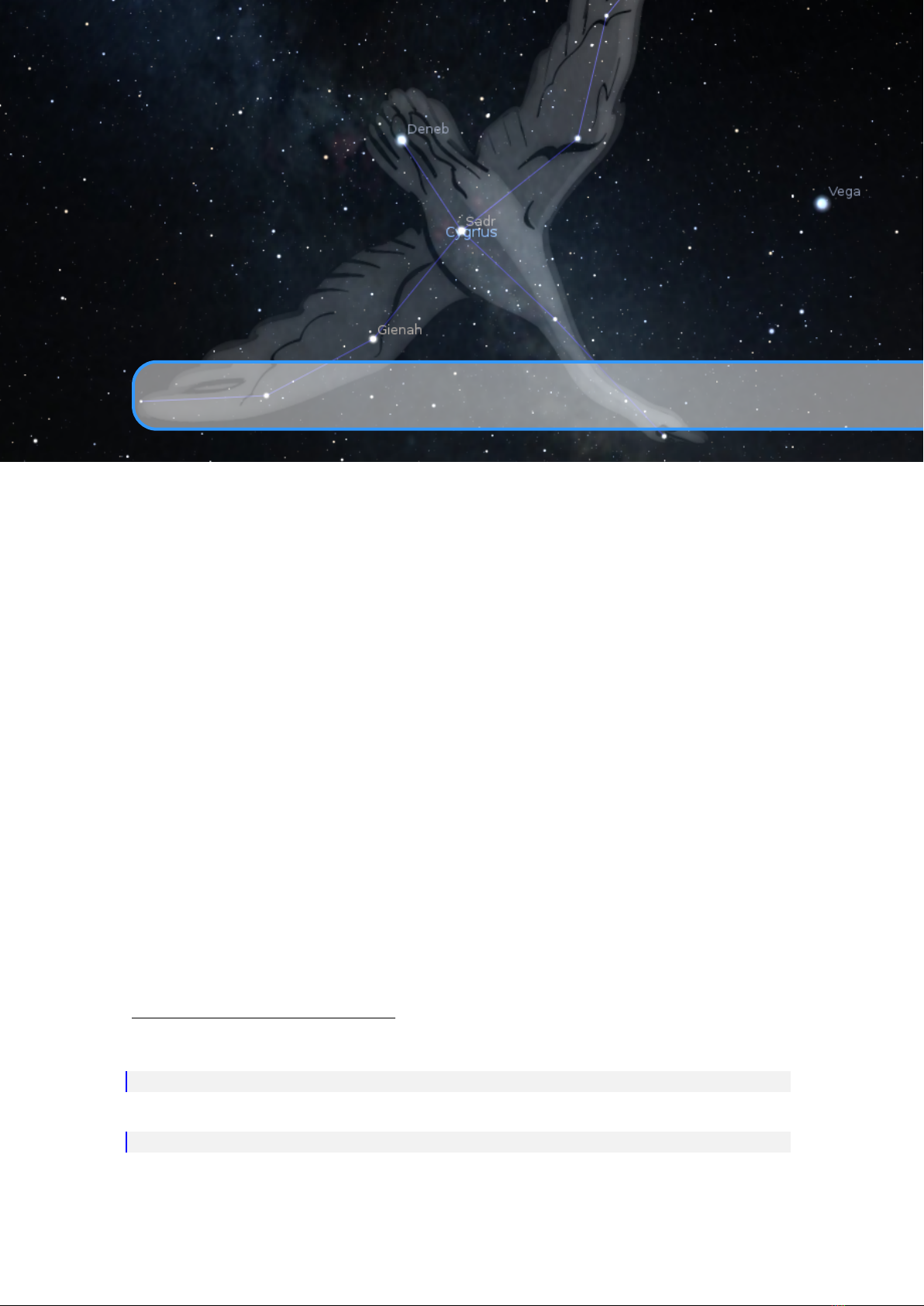
3. A First Tour
Figure 3.1: Stellarium main view. (Combination of day and night views.)
When Stellarium first starts, we see a green meadow under a sky. Depending on the time of day, it is either
a day or night scene. If you are connected to the Internet, an automatic lookup will attempt to detect your
approximate position.
1
At the bottom left of the screen, you can see the status bar. This shows the current observer location,
vertical field of view (FOV), graphics performance in frames per second (FPS) and the current simulation
date and time. If you move the mouse over the status bar, it will move up to reveal a tool bar which gives
quick control over the program.
The rest of the view is devoted to rendering a realistic scene including a panoramic landscape and the
sky. If the simulation time and observer location are such that it is night time, you will see stars, planets and
1
See section 4.2 if you want to switch this off.

12 Chapter 3. A First Tour
the moon in the sky, all in the correct positions.
You can drag with the mouse on the sky to look around or use the cursor keys. You can zoom with the
mouse wheel or the
Page
or
Page
keys.
Much of Stellarium can be controlled very intuitively with the mouse. Many settings can additionally be
switched with shortcut keys (hotkeys). Advanced users will learn to use these shortcut keys. Sometimes
a key combination will be used. For example, you can quit Stellarium by pressing
Ctrl
+
Q
on Windows
and Linux, and
+
Q
on macOS. For simplicity, we will show only the Windows/Linux version. We
will present the default hotkeys in this guide. However, almost all hotkeys can be reconfigured to match
your taste. Note that some listed shortkeys are only available as key combinations on international keyboard
layouts, e.g., keys which require pressing
AltGr
on a German keyboard. These must be reconfigured, please
see 4.8 for details.
The way Stellarium is shown on the screen is primarily governed by the menus. These are accessed by
dragging the mouse to the left or bottom edge of the screen, where the menus will slide out. In case you
want to see the menu bars permanently, you can press the small buttons right in the lower left corner to keep
them visible.
3.1 Time Travel
When Stellarium starts up, it sets its clock to the same time and date as the system clock. However,
Stellarium’s clock is not fixed to the same time and date as the system clock, or indeed to the same speed.
We may tell Stellarium to change how fast time should pass, and even make time go backwards! So the
first thing we shall do is to travel into the future! Let’s take a look at the time control buttons on the right
hand ride of the tool-bar. If you hover the mouse cursor over the buttons, a short description of the button’s
purpose and keyboard shortcut will appear.
Button Shortcut key Description
J
Decrease the rate at which time passes
K
Make time pass as normal
L
Increase the rate at which time passes
8
Return to the current time & date
Table 3.1: Time Travel
OK, so lets go see the future! Click the mouse once on the increase time speed button . Not a
whole lot seems to happen. However, take a look at the clock in the status bar. You should see the time going
by faster than a normal clock! Click the button a second time. Now the time is going by faster than before. If
it’s night time, you might also notice that the stars have started to move slightly across the sky. If it’s daytime
you might be able to see the sun moving (but it’s less apparent than the movement of the stars). Increase the
rate at which time passes again by clicking on the button a third time. Now time is really flying!
Let time move on at this fast speed for a little while. Notice how the stars move across the sky. If you
wait a little while, you’ll see the Sun rising and setting. It’s a bit like a time-lapse movie.
Stellarium not only allows for moving forward through time – you can go backwards too! Click on the
real time speed button . The stars and/or the Sun should stop scooting across the sky. Now press the
decrease time speed button once. Look at the clock. Time has stopped. Click the decrease time speed
button four or five more times. Now we’re falling back through time at quite a rate (about one day every ten
seconds!).

3.2 Moving Around the Sky 13
Time Dragging, Time Scrolling
Another way to quickly change time is time dragging. Press
Ctrl
, press the left mouse button, and slide the
mouse along the direction of daily motion to go forward, or to the other direction to go backward.
Similarly, pressing
Ctrl
and scrolling the mouse wheel will advance time by minutes, pressing
Ctrl
+
and scrolling the mouse wheel will advance time by hours,
Ctrl
+
Alt
by days, and finally
Ctrl
+
+
Alt
by calendar years.
Enough time travel for now. Wait until it’s night time, and then click the real time speed button . If
all works as intended you will now be looking at the night sky.
3.2 Moving Around the Sky
Key Description
Cursor keys Pan the view left, right, up and down
Page
/
Page
,
Ctrl
+
/
Ctrl
+
Zoom in and out
Left mouse button Select an object in the sky
Right mouse button,
Ctrl
+
Clear selected object
Centre mouse button (wheel press) Centre selected object and start tracking
Mouse wheel Zoom in and out
Centre view on selected object
Forward-slash (
/
) Auto-zoom in to selected object
Backslash (
\
) Auto-zoom out to original field of view
+
N
Look towards North (keep altitude)
+
E
Look towards East (keep altitude)
+
S
Look towards South (keep altitude)
+
W
Look towards West (keep altitude)
+
Z
Look towards Zenith (south down)
Alt
+
+
N
Look towards North Celestial Pole
Alt
+
+
S
Look towards South Celestial Pole
Table 3.2: Moving Around the Sky
As well as travelling through time, Stellarium lets you look around the sky freely, and zoom in and out.
There are several ways to accomplish this, listed in table 3.2.
Let’s try it. Use the cursors to move around left, right, up and down. Zoom in a little using the
Page
key, and back out again using the
Page
. Press the
\
key and see how Stellarium returns to the original
field of view (how “zoomed in” the view is), and direction of view.
If you prefer stepwise zooming to fixed values for field of view, table 3.3 lists the keys to reach a certain
field of view.
Most users prefer to move around using the mouse. If you left-click and drag somewhere on the sky, you
can pull the view around.
Hotkey Field of view Hotkey Field of view
Ctrl
+
Alt
+
1
180°
Ctrl
+
Alt
+
6
10°
Ctrl
+
Alt
+
2
90°
Ctrl
+
Alt
+
7
5°
Ctrl
+
Alt
+
3
60°
Ctrl
+
Alt
+
8
2°
Ctrl
+
Alt
+
4
45°
Ctrl
+
Alt
+
9
1°
Ctrl
+
Alt
+
5
20°
Ctrl
+
Alt
+
0
0.5°
Table 3.3: Hotkeys to set fixed vertical fields of view

14 Chapter 3. A First Tour
Another method of moving is to select some object in the sky (left-click on the object), and press the
Space
key to centre the view on that object. Similarly, selecting an object and pressing the forward-slash
key
/
will centre on the object and zoom right in on it.
The forward-slash
/
and backslash
\
keys auto-zoom in and out to different zoom levels depending
on what is selected. If the object selected is a planet or moon in a sub-system with a lot of moons (e.g.
Jupiter), the initial zoom in will go to an intermediate level where the whole sub-system should be visible.
A second zoom will go to the full zoom level on the selected object. Similarly, if you are fully zoomed in
on a moon of Jupiter, the first auto-zoom out will go to the sub-system zoom level. Subsequent auto-zoom
out will fully zoom out and return the initial direction of view. For objects that are not part of a sub-system,
the initial auto-zoom in will zoom right in on the selected object (the exact field of view depending on the
size/type of the selected object), and the initial auto-zoom out will return to the initial FOV and direction of
view.
If you have a touch screen, you can even use one finger directly to drag the sky around and select objects,
and two fingers to zoom. The support for touch screens is incomplete though, and more advanced use of the
program requires the classical operation with keyboard and mouse.
3.3 The Main Tool Bar
Figure 3.2: Night scene with constellation artwork and moon.
Stellarium can do a whole lot more than just draw the stars. Figure 3.2 shows some of Stellarium’s visual
effects including constellation line and boundary drawing, constellation art, planet hints, and atmospheric
halo around the bright Moon. The controls in the main tool bar provide a mechanism for turning on and off
the visual effects.
When the mouse is moved to the bottom left of the screen, a second tool bar becomes visible. All the
buttons in this side tool bar open and close dialog boxes which contain controls for further configuration of
the program. The dialogs will be described in the next chapter.
The position of the toolbars can be changed to any of the four screen corners via the
Toolbar location
drop-down in the
Configuration → Tools → Planetarium options
section.v 26.3
Table 3.4 describes the operations of buttons on the main tool bar and the side tool bar, and gives their
default keyboard shortcuts.
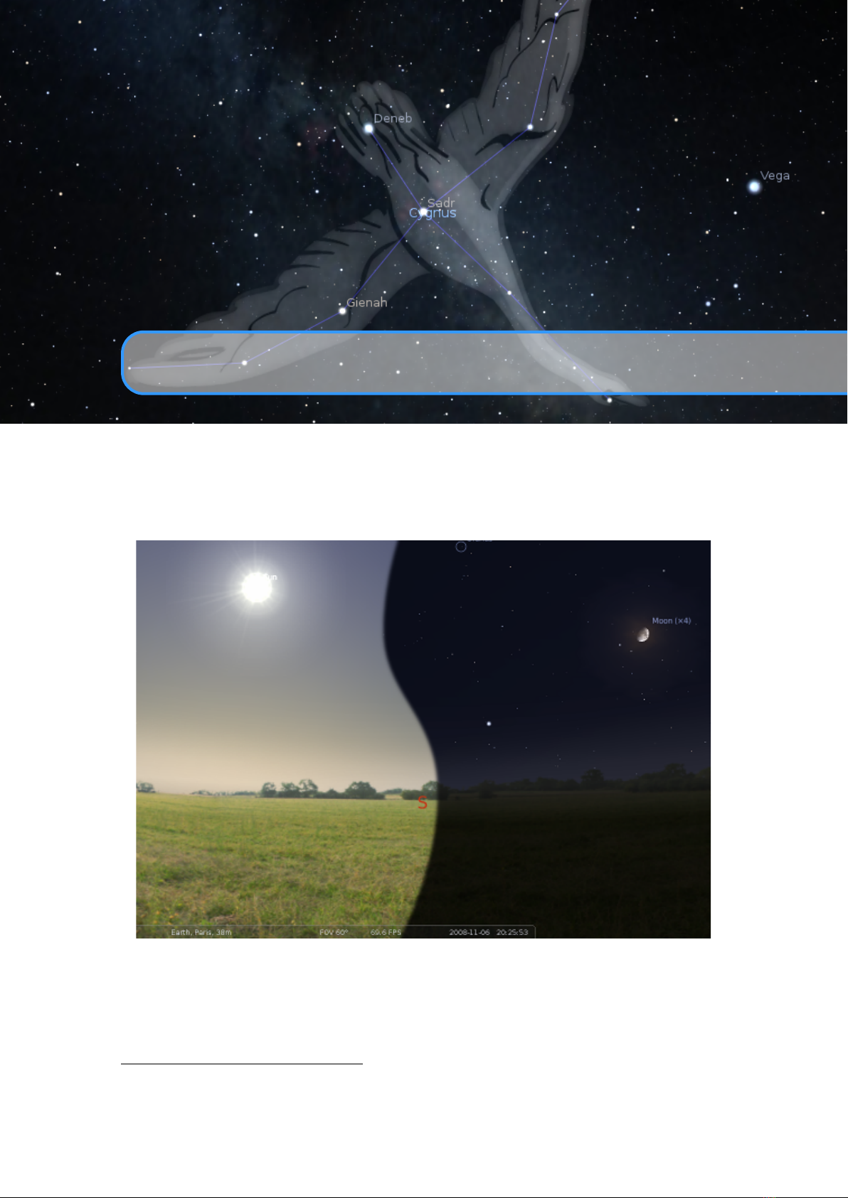
3.3 The Main Tool Bar 15
Feature Button Hotkey Description
Constellations
C
Draw constellations as “stick figures”
Constellation Names
V
Draw name of the constellations
Constellation Art
R
Superimpose artistic representations of
the constellations
Constellation Boundaries
2
B
Draw boundaries of the constellations
Asterisms
2
C
Draw asterism “stick figures”
Asterism Names
2
V
Draw name of the asterisms
Equatorial Grid
E
Draw grid lines for the equatorial coor-
dinate system of date (RA/Dec)
Azimuth Grid
Z
Draw grid lines for the horizontal coor-
dinate system (Alt/Azi)
Galactic Grid
2
Draw grid lines for the galactic coordi-
nate system (Long/Lat)
Equatorial J2000 Grid
2
Draw grid lines for the equatorial
coordinate system at standard epoch
J2000.0 (RA/Dec)
Ecliptic Grid
2
Draw grid lines for the ecliptic coordi-
nate system of date (Long/Lat)
Toggle Ground
G
Toggle drawing of the ground. Turn
this off to see objects that are below the
horizon.
Toggle Cardinal Points
Q
Toggle marking of the North, South,
East and West points on the horizon.
Toggle Compass Marks
2
+
Q
Toggle degree marks along the horizon.
Toggle Atmosphere
A
Toggle atmospheric effects. Most no-
tably makes the stars visible in the day-
time.
Deep-Sky Objects
D
Toggle marking the positions of Deep-
Sky Objects.
Planet Hints
P
Toggle indicators to show the position
of planets.
Nebula images
2
I
Toggle “nebula images”.
Digitized Sky Survey
2
Toggle “Digitized Sky Survey”
(TOAST).
Hierarchical Progressive
Surveys
2
Ctrl
+
Alt
+
D
Toggle “Hierarchical Progressive Sur-
veys”.
Coordinate System
Ctrl
+
M
Toggle between horizontal (Alt/Azi)
& equatorial (RA/Dec) coordinate sys-
tems.
2
This button must be enabled first, see section 4.3.5
16 Chapter 3. A First Tour
Feature Button Hotkey Description
Center Center the view on the selected object
Night Mode
Ctrl
+
N
Toggle “night mode”, which applies a
red-only filter to the view to be easier
on the dark-adapted eye.
Full Screen Mode
F11
Toggle full screen mode.
Bookmarks
2
Alt
+
B
Toggle bookmarks window.
Flip view (horizontal)
2
Ctrl
+
+
H
Flip the image in the horizontal plane.
Flip view (vertical)
2
Ctrl
+
+
V
Flip the image in the vertical plane.
Quit Stellarium
Ctrl
+
Q
Close Stellarium.
Help Window
F1
Show the help window, with key bind-
ings and other useful information
Configuration Window
F2
Show the configuration window
Search Window
F3
or
Ctrl
+
F
Show the object search window
View Window
F4
Show the view window
Time Window
F5
Show the time window
Location Window
F6
Show the observer location window
(map)
AstroCalc Window
F10
Show the astronomical calculations
window
Table 3.4: Stellarium’s standard menu buttons. Those marked
2
must be
enabled first, see section 4.3.3.2.
3.4 Exporting data
3.4.1 Taking Screenshots
You can save what is on the screen to a file by pressing
Ctrl
+
S
. Screenshots are taken in PNG format,
and have filenames like
stellarium-000.png
,
stellarium-001.png
(the number increments to prevent
overwriting existing files).
The screenshots are stored to a directory depending on your operating system, see section 5.1 Files and
Directories. See also section 4.3.5 for more screenshot options.
3.4.2 Copy Information
If you have selected an object and want to use the displayed information elsewhere, you may want to copy
it to the system clipboard with
Ctrl
+
+
C
. In case you want to use its numbers elsewhere, please see
Appendix F for known accuracy limitations.
3.4.3 Scripting
Stellarium is scriptable. You can write your own almanach with it. See chapter 17 for details.
3.5 Observing Lists (Bookmarks) 17
3.5 Observing Lists (Bookmarks)
You can store your favourite objects or views in observing lists. Press
Alt
+
B
or to call up the
dialog. A bookmarks file from previous versions will be imported and converted to the new format. You can
however create an arbitrary number of lists.
The list display shows all entries from the current list. A double click on an entry selects the object.
To add/remove an object to/from the list, press
Edit list
. This changes the view. Highlight (select) your
object in the sky and press
Add object
. To remove an object from a list, select its entry in the list and press
Remove object
.
Sometimes storing the object alone is not enough. Interesting views like planet conjunctions or eclipses
require at least a time entry, if not a particular location. Likewise, the displayed landscape may be nice to
restore. Additionally, the field of view may be relevant. To store these data and later retrieve them, use the
respective checkboxes.
You can also export the current list or all lists with the according button, or import such an exported list
on another system. To export the current list, keep the default
.sol
file type in the filename dialog. To export
all your lists, use the
.ol
file type in the filename dialog. Lists are identified with an Universally Unique
Identifier (UUID) which we call OLUD (Observing List Unique Identifier). On importing a list, existing lists
with the same OLUD may be replaced after a warning. During editing, storing a list with an existing name is
prevented. The list import may however import a list with an existing name as long as the OLUD is different.
You may want to change one of the duplicate list names after import. To transfer all your lists to another
system, export them as
.ol
file, or copy, rename and import (or just copy, to replace the existing) the full file
observingLists.json from the data/ subdirectory of your user directory (see section 5.1).
3.6 Custom Markers
You can set temporary markers anywhere in the screen. These may be useful for various purposes but cannot
be stored.
Actions Description
Shift
& left click Add custom marker
Shift
& right click Delete the one closest marker to mouse cursor
Alt
+
& right click Delete all custom markers
3.7 Speech Output
Sometimes you may have dimmed down your field laptop or the font may be too small. Object information
v 25.4
can also be output audibly by a Text-to-Speech engine. After object selection, press
Shift
+
R
to let a voice
read ot to you. See section 4.3.6 for details and configuration.
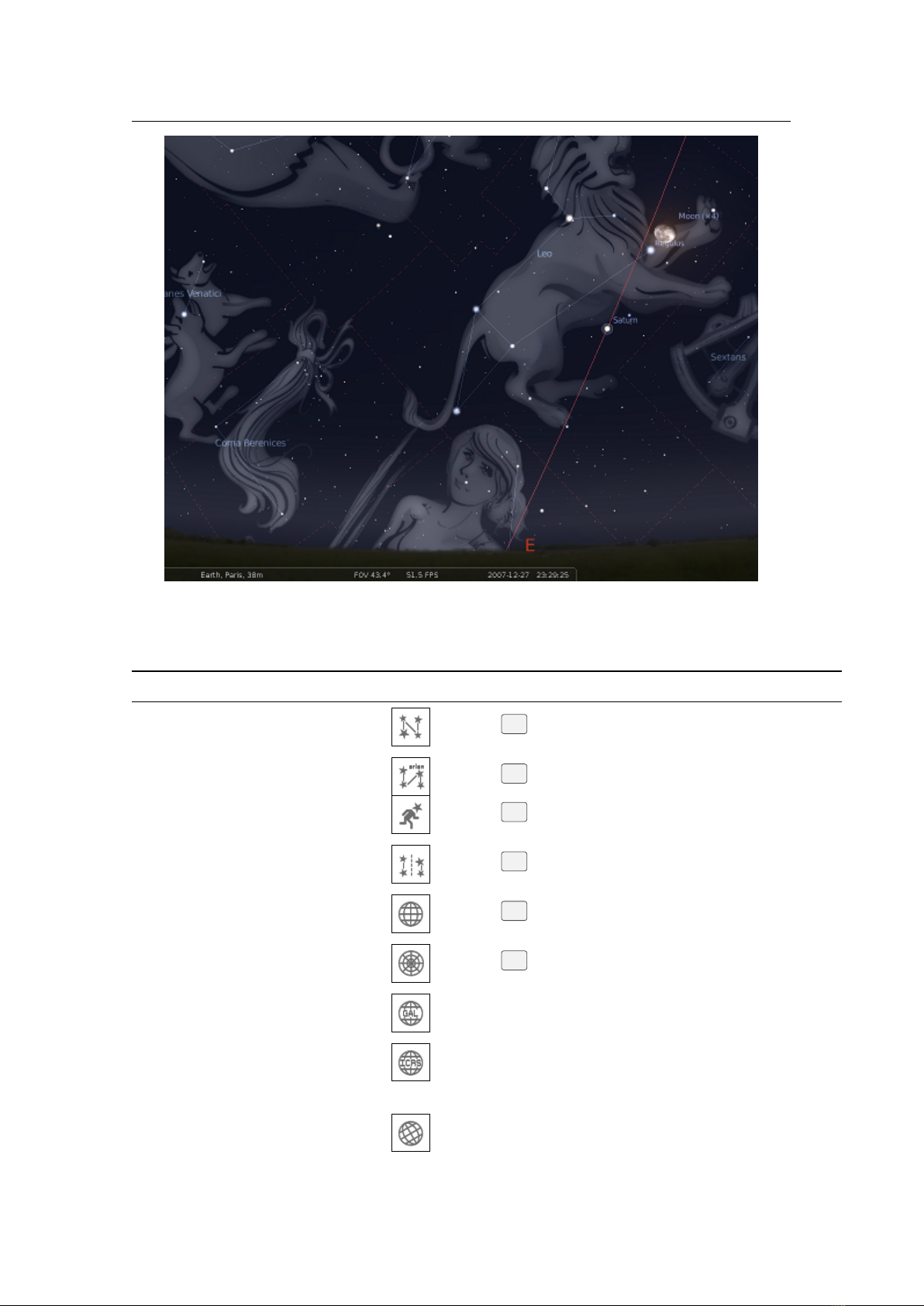
4. The User Interface
This chapter describes the dialog windows which can be accessed from the left menu bar.
Most of Stellarium’s settings can be changed using the view window (press or
F4
) and the
configuration window (
or
F2
). Most settings have short labels. To learn more about some settings,
more information is available as tooltips, small text boxes which appear when you hover the mouse cursor
over a button.
1
You can drag the windows around, and the position will be used again when you restart Stellarium. If
this would mean the window is off-screen (because you start in windowed mode, or with a different screen),
the window will be moved so that at least a part is visible.
Some options are really rarely changed and therefore may only be configured by editing the configuration
file. See 5.4 The Main Configuration File for more details.
4.1 Setting the Date and Time
Figure 4.1: Date and Time dialog
In addition to the time rate control buttons on the main toolbar, you can use the date and time window
(open with the button or
F5
) to set the simulation time. The values for year, month, day, hour, minutes
and seconds may be modified by typing new values, by clicking the up and down arrows above and below
the values, and by using the mouse wheel.
The other tab in this window allows you to see or set Julian Day and/or Modified Julian Day numbers
(see 18.4.2).
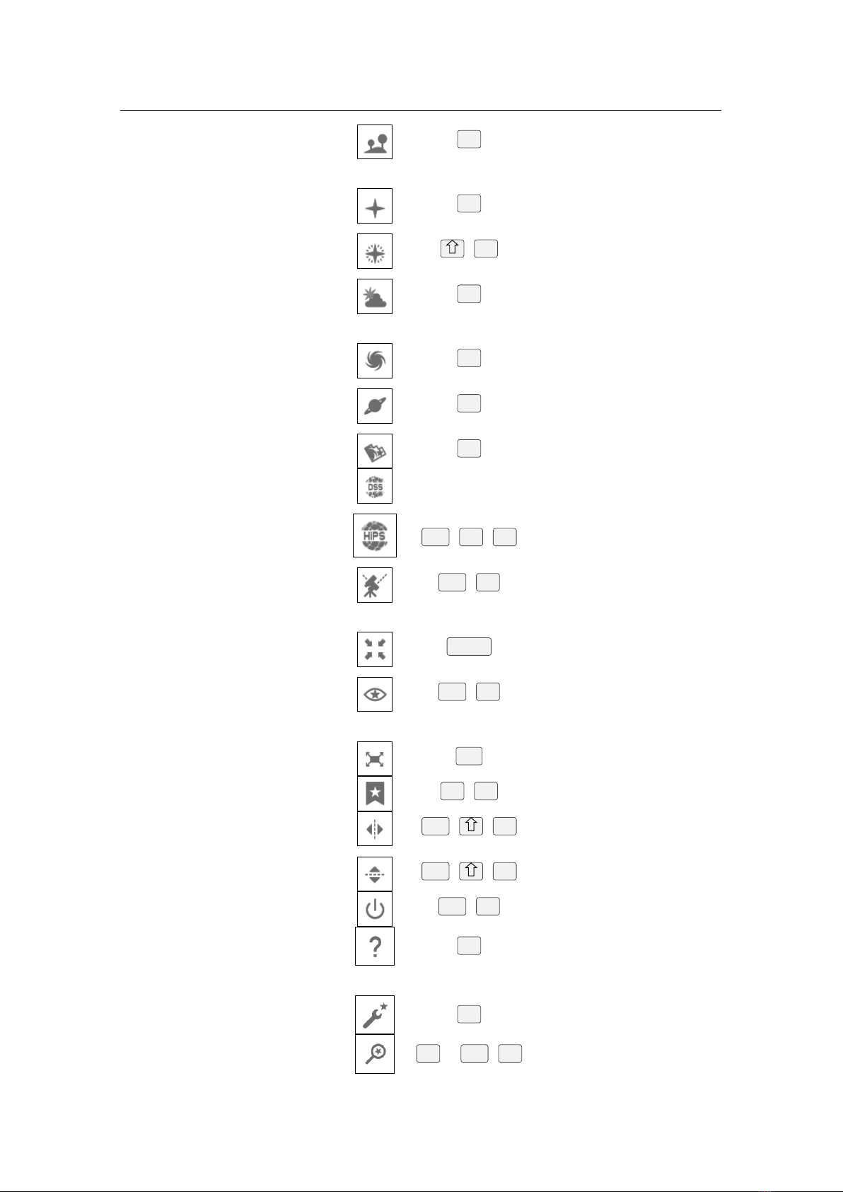
20 Chapter 4. The User Interface
Figure 4.2: Location window
4.2 Setting Your Location
The positions of the stars in the sky is dependent on your location on Earth (or other planet) as well as the
time and date. For Stellarium to show accurately what is (or will be/was) in the sky, you must tell it where
you are. You only need to do this once – Stellarium can save your location so you won’t need to set it again
until you move.
After installation, Stellarium uses an online service which tries to find your approximate location based
on the IP address you are using. This seems very practical, but if you feel this causes privacy issues, you
may want to switch this feature off. You should also consider switching it off on a computer which does not
move, to save network bandwidth.
To set your location more accurately, or if the lookup service fails, press
F6
to open the location window
(Fig. 4.2). There are a few ways you can set your location in this dialog:
1. Just click on the map.
2.
Search for a city where you live using the search edit box at the top right of the window, and select
the right city from the list.
3.
Click on the map to filter the list of cities in the vicinity of your click, then choose from the shortlist.
4. Enter a new location using the longitude, latitude and other data.
5.
Click on
Get Location from GPS
if you have a GPS receiver. You activate a periodic request for GPS
fixes. After a few seconds, the button should change color and give a textual feedback. Green indicates
a good location fix, yellow indicates a 2D-fix only, which means altitudes are not available. (Leave the
GPS device running for a few minutes and/or search a place with better sky view.) You could leave it
running if you are operating a fast-moving observatory platform, but rather switch it off when you see
a good fix, so that other programs can use the serial GPS connection. Red signals an error, and further
positions are not retrieved but the button is reset. You may press the button again to start over.
Sometimes you have to try several times or let it run for a while to get a green button indicating a
valid 3D fix including altitude. See section 5.5.4 for configuration details.
On Windows, if there is no GPS device, a system location service will be queried as fallback.v 1.0
If you want to use the current location permanently, click on the “use as default” checkbox, disable “Get
location from Network”, and close the location window.
Two settings may influence the landscape when changing locations:
Auto select landscapes
When changing the planet, a fitting landscape panorama will be shown when
available. Also, when clicking on the earth map, a zero-altitude landscape is displayed in the
v 23.2
1
Unfortunately, on Windows 7 and later, with some Nvidia and AMD GPUs in OpenGL mode, these tooltips
sometimes do not work. Sometimes it is enough to leave fullscreen mode to see them.
4.3 The Configuration Window 21
approximate color of that location (taken from the map).
Auto-enable atmosphere
When changing planet during location change, the atmosphere will be switched
as required.
As a reverse functionality, loading landscapes may also change location. See section 4.4.5.
4.2.1 Time Zones
Locations in Stellarium’s location database include their respective time zone. When you click on a location
in the list, the time should be shown in the respective time zone. If daylight time rules exist and you have
selected “Enable daylight saving time”, also this abomination of modern civilisation is respected. Most users
will require to have this setting active.
When you select “Use custom time zone”, you can select other time zones. Those that start with UTC
have no daylight time rules.
Time zones were introduced in the 19th century, originally for purposes of railway traffic synchronization.
The first such action was taken in 1847, and therefore Stellarium by default will present Local Mean Solar
Time (LMST) for dates before 1847, and ignore all configured time zones unless you deliberately activate
“Use custom time zone”. The history of time zones and their rules is very complicated, though, and Stellarium
should not be expected to find the exact date when time zone use was introduced at a certain location or
country. Just be sure to use LMST when replaying historical observations before the 20th century.
For even earlier observations, you can also set Local True Solar Time (LTST), which is the time given
by sundials. Here, 12 o’clock is the time when the sun transits the meridian, strictly, daily. The difference
between LMST and LTST is called equation of time. See section 13.2 for more information.
When you click on the map to set your location, Stellarium has currently no way to guess the timezone of
the coordinate pair. In this case, Local Mean Solar Time is presented, which only depends on longitude and
was the “normal” time before the development of time zones. Either select a city from the list or manually
select a time zone.
4.2.2 Geographical Regions
The world is split into political entities called “countries”. Humans have an unappealing tendency of
fighting over the question to which country some territories should be counted. Stellarium is an astronomy
program which labels coordinates of locations like cities with a name. Earlier editions of Stellarium used
countries as further superordinate entities to locations for identification purposes. In consequence to much
unnecessary and unfriendly discussion we decided to completely drop the petty-minded assignment of
political country names to locations in favour of geographical regions. There is only one known habitable
planet, one humankind, and one sky. Stellarium users should overcome borders!
For the “region” classification of sky cultures we use the same regions (see 9.2.1), and we follow the
UN M49 geoscheme
2
with extensions for other planets.
4.2.3 Observers
In the list of Planets you can find entries called Solar System Observer, Jupiter Observer and similar for
each major planet that has moons: Earth, Mars, Jupiter, Saturn, Uranus, and Neptune. These are specialized
locations. When switching to them, you will find yourself looking onto the respective observed object (Sun,
Jupiter, . . . ) from somewhat above the plane of the Solar system. By pressing
Alt
+
/
Alt
+
you can
rotate around a vertical axis through the observed object. Likewise, by pressing
Alt
+
/
Alt
+
you can
change the latitude of observation. Finally, with
Alt
+
Home
/
Alt
+
End
you can change the distance from
the observed object.
4.3 The Configuration Window
The configuration window contains general program settings, and many other settings which do not concern
specific display options. Press the tool button or
F2
to open.
4.3.1 The Main Tab
The Main tab in the configuration window (Fig. 4.3) provides control for changing the program language.
The next setting group allows to enable using DE430/DE431 and DE440/DE441 ephemeris files. These
files have to be installed separately. Most users do not require this. See section 5.5.3 if you are interested.
2
https://unstats.un.org/unsd/methodology/m49/

22 Chapter 4. The User Interface
Figure 4.3: Configuration Window: Main Tab
The tab also provides the buttons for saving the current view direction as default for the next startup, and
for saving the program configuration: most display settings have to be explicitly stored to make a setting
change permanent. If you prefer, you can activate
Immediate Save
. Then all settings changes will be stored
v 24.4
immediately and the program will use them the next time you launch it. Language and font settings have
to be stored explicitly with the buttons next to their settings to protect you from unwanted surprises. To
permanently set this mode, use
Save settings
a final time.
4.3.2 The Information Tab
Figure 4.4: Configuration Window: Information Tab
The Information tab (Fig. 4.4) allows you to set the type and amount of information displayed (left column)
or output by speech (right column; see 4.3.6) about a selected object. The Radio buttons on the top of the
v 25.4
dialog allow quick selection of some useful configurations for display.
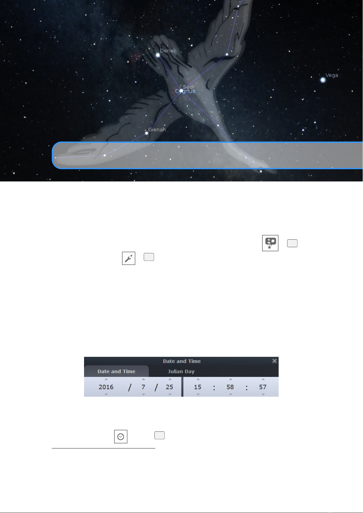
4.3 The Configuration Window 23
4.3.3 The Extras Tab
Figure 4.5: Configuration Window: Extras Tab
The Extras tab (Fig. 4.5) allows you to customize information displayed about a selected object, download
more star catalogs and also allows to hide or show additional buttons in the lower button bar.
4.3.3.1 Customization of information displays
The information display can be tweaked a bit with the options found in the GUI section “Additional
information settings”.
Use mag/arcsecˆ2 for surface brightness instead of mag/arcminˆ2.
Short notation for units of surface brightness symbolic abbreviation.
Designations for celestial coordinate systems Use symbols like
α, δ instead of textual labels.
Tabular output for coordinates and time uses a more eye-friendly layout.
Use decimal degrees You can toggle usage of decimal degree format for coordinates.
Azimuth from South Some users may be used to counting azimuth from south.
Allow negative hour angles Count hour angles −12h. . . 12h instead of 0h. . . 24h. v 25.4
Polar distance, not declination Used by some telescopes. Using label p or PD instead of
δ. v 25.4
4.3.3.2 Customization of button visibility on bottom toolbar
If your screen is too narrow to show all buttons or you simply don’t need them because you prefer the
keyboard shortcuts, you can choose your optimal setup. The selection of buttons is stored immediately.
Constellation boundaries You can toggle display of constellation boundaries with this button.
Asterism lines You can toggle display of asterism lines with this button.
Asterism labels You can toggle display of asterism labels with this button.
Ecliptic grid You can toggle display of ecliptic coordinate grid with this button.
ICRS grid
You can toggle display of the International Coordinate Reference System (equatorial J2000
coordinate grid) with this button.
Galactic grid You can toggle display of galactic coordinate grid with this button.
Cardinal points You can toggle display of the “Cardinal points” button.
Compass marks You can toggle display of the “Compass marks” button.
Night mode You can toggle display of the nightmode button.
Centering button You can toggle display of the “Center on selected object” button.
Fullscreen button You can toggle display of the fullscreen button.
Quit button You can toggle display of the button to quit Stellarium.
Nebula background You can toggle display of DSO photographs with this button.
Flip buttons
When enabled, two buttons will be added to the main tool bar which allow the main view to
be mirrored in the vertical and horizontal directions. This is useful when observing through telecopes
which may cause the image to be mirrored.
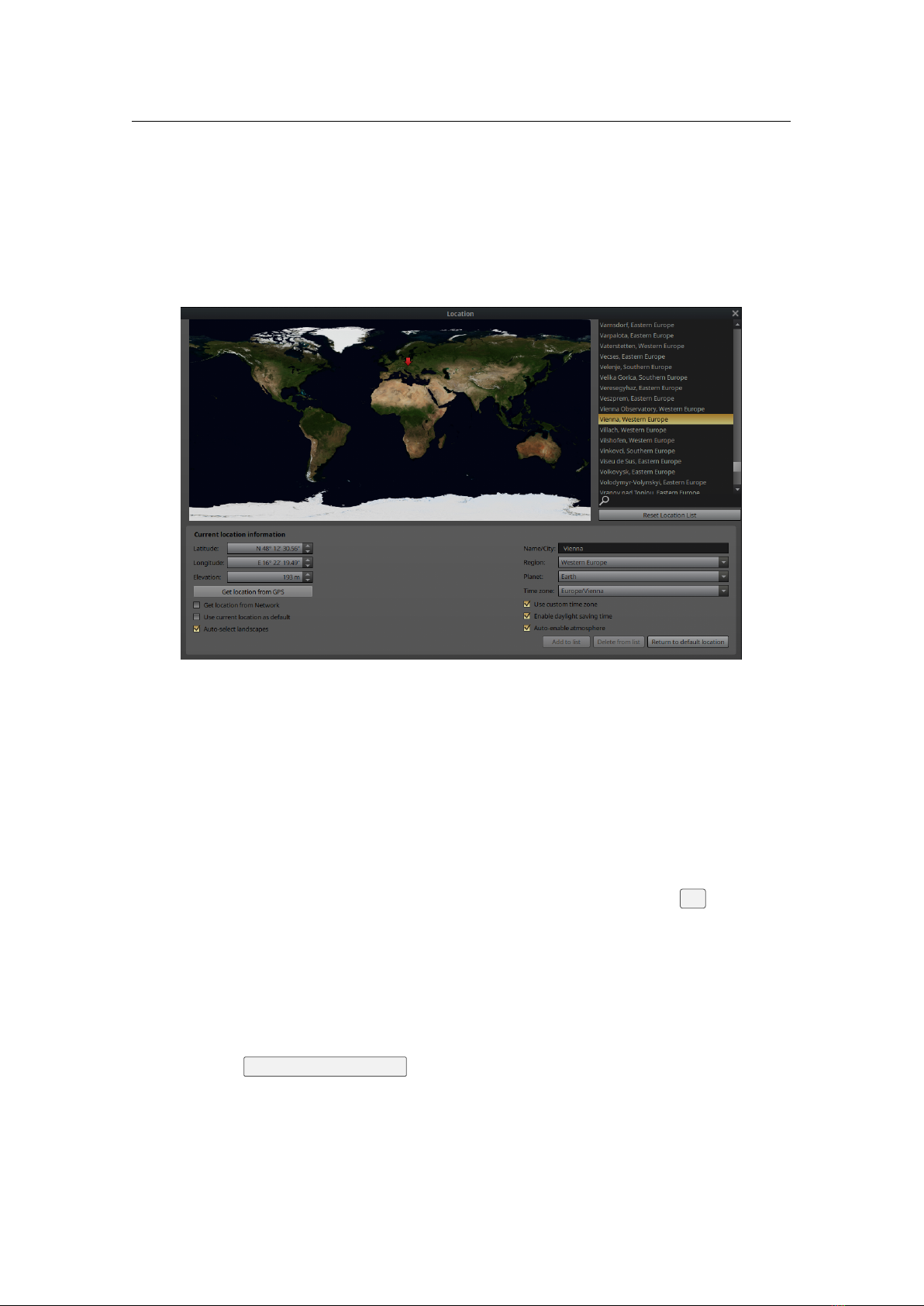
24 Chapter 4. The User Interface
DSS survey You can toggle display of Digitized Sky Survey with this button (see section 10.4).
HiPS Surveys
You can toggle display of Hierarchical Progressive Surveys with this button (see section
4.4.7).
Bookmarks You can enable display of Bookmarks (Observing Lists) dialog with this button.
Use buttons background Applies a gray background under the buttons on the bottom bar.
4.3.3.3 Download more star catalogs
Stellarium comes with enough stars for casual stargazing with the unaided eye or binoculars. If you have a
telescope and want to see more stars, here you can download more catalogs. (See Appendix C)
4.3.4 The Time Tab
Figure 4.6: Configuration Window: Time Tab
The Time tab (Fig. 4.6) allows to specify what simulation time should be used when the program starts:
System date and time Stellarium will start with the simulation time equal to the operating system clock.
System date at
Stellarium will start with the same date as the operating system clock, but the time will be
fixed at the specified value. This is a useful setting for those people who use Stellarium during the day
to plan observing sessions for the upcoming evening.
Other some fixed time can be chosen which will be used every time Stellarium starts.
The middle field allows specify display formats for date and time on bottom toolbar:
JD Stellarium will display Julian Days (JD).
Date and time Stellarium will display date and time in selected format.
The lowest field allows selection of the correction model for the time correction
∆T
(see section 18.4.3).
Default is “Modified Espenak and Meeus (2006, 2014, 2023)”. Please use other values only if you know
what you are doing.
4.3.5 The Tools Tab
The Tools tab (Fig. 4.7) contains planetarium options (like enabling/disabling of keyboard shortcuts for
panning and zooming the main view) and options for screenshots.
Spheric mirror distortion
This option pre-warps the main view such that it may be projected onto a
spherical mirror using a projector. The resulting image will be reflected up from the spherical mirror
in such a way that it may shine onto a small planetarium dome (or even just the ceiling of your dining
room), making a cheap planetarium projection system.
Disc viewport
This option masks the main view producing the effect of a telescope eyepiece. It is also
useful when projecting Stellarium’s output with a fish-eye lens planetarium projector.

4.3 The Configuration Window 25
Figure 4.7: Configuration Window: Tools Tab
Gravity labels
This option makes labels of objects in the main view align with the nearest horizon. This
means that labels projected onto a dome are always aligned properly.
Auto zoom out returns to initial direction of view
When enabled, this option changes the behavior of the
zoom out key
\
so that it resets the initial direction of view in addition to the field of view.
Enable keyboard navigation
, i.e. moving the view with cursor keys. The tool button calls the keyboard
configuration panel. (See section 4.8.)
Enable mouse navigation , i.e. mouse dragging.
Enable mouse zooming use mouse wheel to zoom field of view.
Mouse cursor timeout
You can decide whether, and when, the mouse cursor should disappear from view
when not moved.
Include Topocentric coordinates
If you require planetocentric coordinates, you may switch this off.
Usually it should be enabled. (See 18.9.1)
Nutation
Compute the slight wobble of earth’s axis. This feature is active only about 500 years
around J2000.0.
Aberration
Add effect of annual aberration of light to the object’s position (see 18.10). Note:
This also influences the displayed position in the J2000 frame! For didactic purposes you can
exaggerate the effect by up to 5×.
Overwrite text color
— enabling this option will ignore the color settings for each celestial object and
enable one color for text on the info panel for all celestial objects. By default Stellarium uses white
color for this option, but you may re-define it through a color chooser.
Set keyboard focus to day input
— you may use this option to force setting the keyboard focus on the day
input field in the Date and Time dialog.
Important note: the focus in the sky will be lost when you open the Date and Time dialog after
enabling this option.
Use kinetic scrolling
Text fields in dialogs can either be moved on sidebar handles (with this switch
disabled) or by dragging the text itself (enabled), as it is known from touch-enabled devices like
smartphones.
Dithering options to allow select better simulation of sky on different hardware.
Indication for mount mode
You can activate the short display of a message when switching type of used
mount.
Info text color at daylight
— this is a color chooser for defining the text color for the info panel at daylight
to increase the contrast of the text. By default Stellarium use black color.
4.3.5.1 Toolbar position
v 26.3
The Toolbar location drop-down in the Planetarium options section of the Tools tab lets you dock both
toolbars to any of the four screen corners:
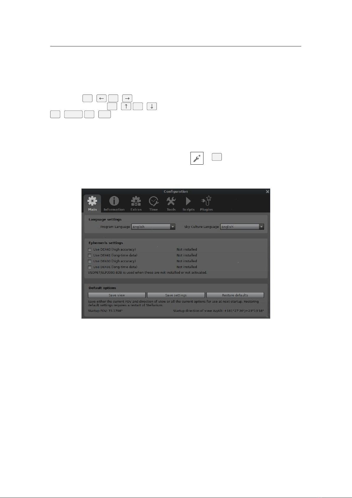
26 Chapter 4. The User Interface
Bottom-left Default position: tool button bar at the bottom, dialog button bar on the left.
Bottom-right Tool button bar at the bottom, dialog button bar on the right.
Top-left
Tool button bar at the top, dialog button bar on the left. When the tool button bar is at the top, the
status row (location, FOV, date/time) moves below the buttons so it remains visible when the bar is
partially hidden.
Top-right Tool button bar at the top, dialog button bar on the right.
The selection is saved as
toolbar_corner
(integer 0–3) in the [gui] section.
Multithreading
For every frame, the positions of all planets and minor bodies of the Solar system are computed. Most of the
other time between frame updates is needed for the actual frame drawing, and waiting for the next frame
cycle if you have deliberately set a low frame rate (useful to conserve energy; see below). If you have many
thousands of solar system objects and a moderately new computer, you may feel that Stellarium becomes
slow (few frames/second) but see that mostly only one core of your CPU seems to be busy. You can try to
v 24.3
distribute the computation of solar system bodies to more CPU cores. But take note, thread synchronization
(combining all results ahead of drawing) takes its time, so it pays off only when your solar system is really
large. With more than 1000 objects, we recommend starting with 1 additional thread. Even with 25.000
objects, assigning more than 4 additional threads on a 20-core CPU does not show any further gain. Frame
drawing is still performed by the main thread, and too many objects still slow down the program. Just try out
what works best on your system.
Framerate intent
The pace of screen updates (frames per second, FPS) depends on several factors: CPU speed, graphics card
speed, screen size, number of displayed objects and grids, etc. As is common for interactive programs,
the main program thread runs on a single core also on a multicore system. For running Stellarium, a CPU
with few but fast cores will appear faster in total than a multicore system at slower CPU cycles. High-end
systems may deliver needlessly high framerates, at cost of energy consumption. The maximum FPS setting
limits the frame rate when Stellarium is interactively operated (zoomed, panned, settings switched, etc.)
After a few seconds, when Stellarium is not interactively operated, it falls back to a minimum FPS setting
to conserve energy. Of course, when the system cannot even reach this FPS, the factual FPS will be lower
and the system may be overloaded. Keep in mind that the minimum setting also applies to running scripts
(non-interactively).
Font size and font selection
You can change the font sizes for on-screen text and GUI dialogs separately. For some purposes like
presentations it may be helpful to enlarge screen font size while keeping GUI font regular, or vice versa. It
also depends on your screen size whether all the object info fits on screen. This may also depend on the
writing system and installed font. If you are using a non-Western character system and the default font
looks bad, you can select another system font. For this, edit
config.ini
(see chapter 5.1): locate the
[gui]
section and set the key
flag_font_selection=true
. On next start of Stellarium, you will find two
elements for font selection: one allows you to pre-select a writing system, the other will then allow selection
of a font installed in your system that includes the characters used in the selected writing system. When you
have found the best font, store your settings here or on the Main tab (see section 4.3.1), and you may edit
config.ini again to disable the font selection switches.
Screenshots
You can set the directory where screenshots will be stored, and also whether you want screenshots sized
like Stellarium’s window or some other, likely larger size. The maximum possible size depends on your
hardware.
4096× 4096
should be possible on most PCs, others may even create
16384× 16384
images. The
vertical field of view will be the same as in the current view.
You can also set the file format. The exact selection depends on platform and version of the underlying
Qt framework. Notable formats are PNG (lossless), JPG (lossy), JPEG (higher quality JPG), BMP (Windows
Bitmap), WEBP, TIF (LZW compressed), TIFF (uncompressed), PBM, PGM, PPM, XBM, XPM, and ICO
(thumbnails).
Some printing workflows require particular DPI (dots per inch) settings stored in the screenshots. You
can configure DPI which will be stored in the image metadata. The intended print size in
mm
is shown in
the tooltip of the dpi spinner.
4.3.6 The Speech Tab
The Speech tab (Fig. 4.8) allows configuring speech output.
3
You can select some speech engine, then
v 25.4
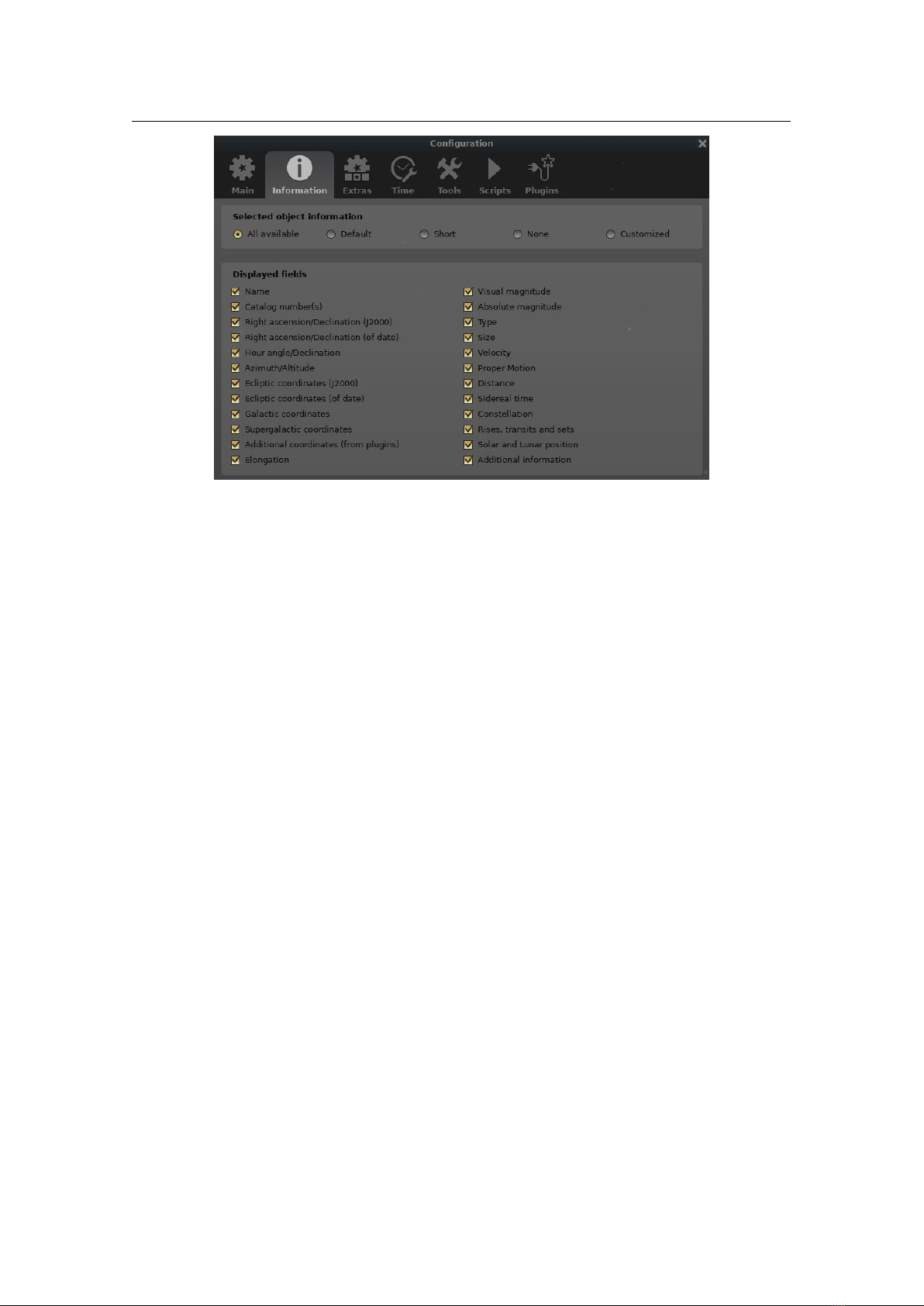
4.4 The View Settings Window 27
Figure 4.8: Configuration Window: Speech Tab
(hopefully) a list of voices for your user language becomes available from which you can choose. You can
influence pitch and speed (Rate) and balance volume against your system volume. Then test the content of
the text box with the
▶ Say
, or cut this off via
∎ Stop
.
Speech output is available for data of the currently selected object. In the Information tab (see 4.3.2), the
right checkbox colums let you select those information bits which should be output by voice. Most users
will keep coordinate readings off, but some physical or morphological data may be interesting to listen to.
The default hotkey for speech output is
Shift
+
R
. Pressing it another time will cut off narration.
Also the long texts in the Landscape (see 4.4.5) and Skyculture (4.4.6) tabs of the View Settings dialog
can be narrated with the
▶ Read text
/
∎ Stop
buttons near the respective text boxes.
4.3.7 The Scripts Tab
The Scripts tab (Fig. 4.9) allows the selection of pre-assembled scripts bundled with Stellarium that can be
run (See chapter 17 for an introduction to the scripting capabilities and language). This list can be expanded
with your own scripts as required. See section 5.2 where to store your own scripts.
When a script is selected it can be run by pressing the arrow button and stopped with the stop button.
With some scripts the stop button is inhibited until the script is finished.
Scripts that use sound or embedded videos will need a version of Stellarium configured at compile time
with multimedia support enabled. It must be pointed out here that sound or video codecs available depends
on the sound and video capabilities of you computer platform and may not work.
4.3.8 The Plugins Tab
Plugins (see chapter 12 for an introduction) can be enabled here (Fig. 4.10) to be loaded the next time you
start Stellarium. When loaded, many plugins allow additional configuration which is available by pressing
the
configure
button on this tab.
4.4 The View Settings Window
The View settings window controls many display features of Stellarium which are not available via the main
toolbar.
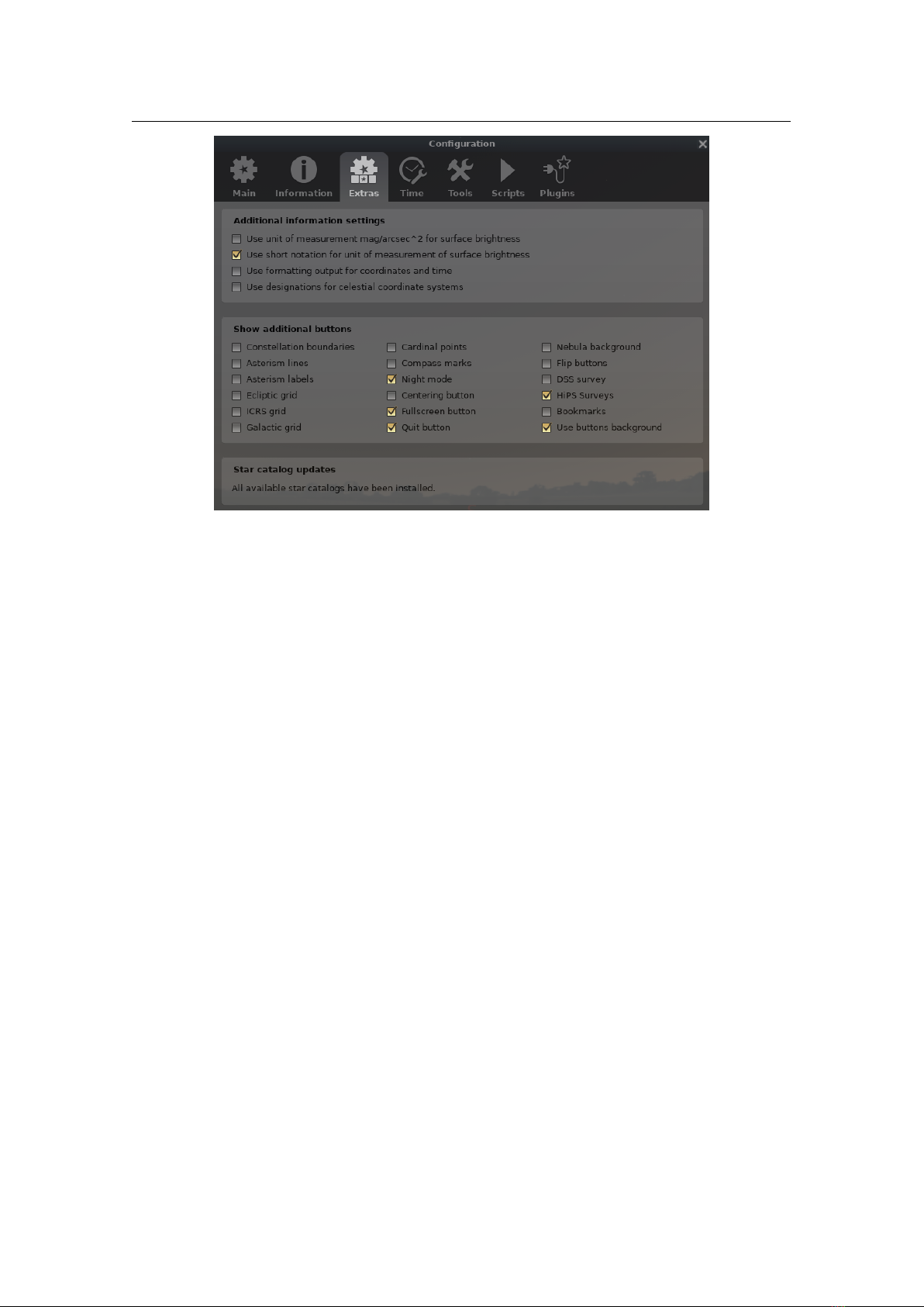
28 Chapter 4. The User Interface
Figure 4.9: Configuration Window: Scripts Tab
Figure 4.10: Configuration Window: Plugins Tab
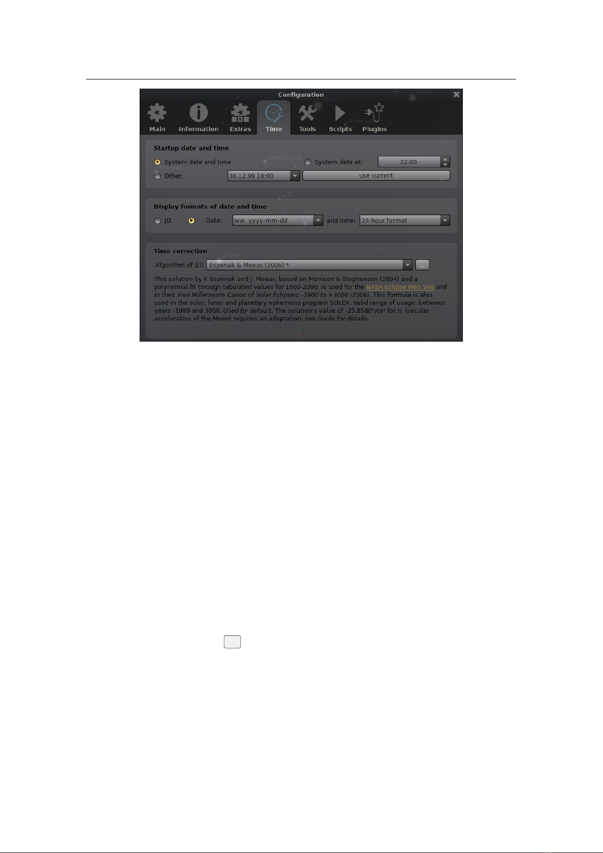
4.4 The View Settings Window 29
Figure 4.11: View Settings Window: Sky Tab
4.4.1 The Sky Tab
The Sky tab of the View window (Fig. 4.11) contains settings for changing the general appearance of the
main sky view and projections. Some highlights of sky field:
Dynamic eye adaptation
When enabled this feature reduces the brightness of faint objects when a bright
object is in the field of view. This simulates how the eye can be dazzled by a bright object such as the
moon, making it harder to see faint stars and galaxies.
Light pollution
In urban and suburban areas, the sky is brightened by terrestrial light pollution reflected in
the atmosphere. Stellarium simulates light pollution and lets the user configure how bright the night
sky is. There are several ways to set it up:
Automatic from locations database
option makes Stellarium find sky brightness from its locations
database and simulate light pollution without any further user input.
Manual
mode lets the user choose the amount of light pollution by moving a slider. To make it easier
to orient in the resulting amount of light pollution, a tooltip will show the classification of the
sky according to the Bortle Dark Sky Scale (See Appendix B for more information), as well as
the naked-eye limiting magnitude.
Manual from SQM
mode lets one enter the reading of a Sky Quality Meter. Stellarium can accept it
in several units: physical (
cdm
2
,
mcdm
2
,
µcdm
2
) as well as astronomical,
magarcsec
2
. To
enter a value, first choose the unit, and then type the number into the spinbox.
Solar altitude for Twilight Finder
You can configure shortcut keys to go to the time when the sun reaches
this altitude below the mathematical horizon. See section 4.8.1.
Shooting stars
Stellarium has a simple meteor simulation option. This setting controls how many shooting
stars will be shown. Note that shooting stars are only visible when the time rate is 1, and might not
be visible at some times of the day. Meteor showers can be simulated using a dedicated plugin (see
section 14.6).
Some highlights of the stars field:
Absolute scale
is the size of stars as rendered by Stellarium. If you increase this value, all stars will appear
larger than before.
Relative scale
determines the difference in size of bright stars compared to faint stars. Values higher than
1.00 will make the brightest stars appear much larger than they do in the sky. This is useful for creating
star charts, or when learning the basic constellations.
Twinkle
controls how much the stars twinkle when atmosphere is enabled (scintillation, see section 19.13.2.1).
Since v0.15.0, the twinkling is reduced in higher altitudes, where the star light passes the atmosphere
in a steeper angle and is less distorted.
Limit magnitude
Inhibits automatic addition of fainter stars when zooming in. This may be helpful if you
are interested in naked eye stars only.
3
This fully depends on capabilities of the operating system and is not available for builds/platforms with Qt version
less than 6.4.
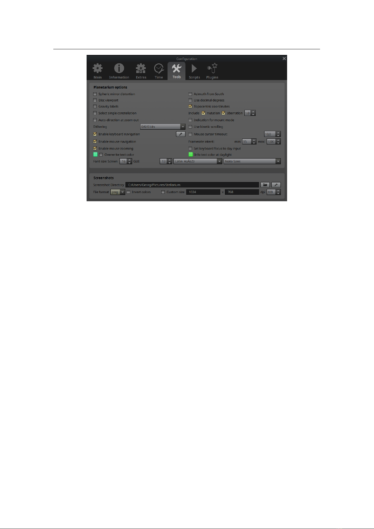
30 Chapter 4. The User Interface
Labels and markers
you can independently change the amount of labels displayed for stars. The further to
the right the sliders are set, the more labels you will see. Note that more labels will also appear as you
zoom in.
Use designations for screen labels
— when this option is enabled you will see in the sky (on-screen labels)
only scientific designations (catalog numbers) of the stars instead of their common names. To
customize the on-screen labels we added 3 additional options
4
— Dbl. stars, Var. stars and HIP
— which will show, in this sequence of preference, the first available occurrence of the traditional
designations of double stars, variable stars or HIP numbers, respectively.
4.4.1.1 The Projections field
Selecting items in this list changes the projection method which Stellarium uses to draw the sky (Snyder,
1987). Options are:
Perspective
Perspective projection maps the horizon and other great circles like equator, ecliptic, hour lines,
etc. into straight lines. The maximum field of view is 150°. The mathematical name for this projection
method is gnomonic projection.
Stereographic
Stereographic projection has been known since antiquity and was originally known as the
planisphere projection. It preserves the angles at which curves cross each other but it does not preserve
area. Else it is similar to fish-eye projection mode. The maximum field of view in this mode is 235°.
Fish-Eye
Stellarium draws the sky using azimuthal equidistant projection. In fish-eye projection, straight
lines become curves when they appear a large angular distance from the center of the field of view
(like the distortions seen with very wide angle camera lenses). This is more pronounced as the user
zooms out. The maximum field of view in this mode is 180°.
Orthographic
Orthographic projection is related to perspective projection, but the point of perspective is
set to an infinite distance. The maximum field of view is 180°.
Equal Area
The full name of this projection method is Lambert azimuthal equal-area projection. It
preserves the area but not the angle. The maximum field of view is 360°.
Hammer-Aitoff
The Hammer projection is an equal-area map projection, described by ERNST VON
HAMMER (1858–1925) in 1892 and directly inspired by the Aitoff projection. The maximum field of
view in this mode is 360°.
Mollweide
The Mollweide projection is a pseudocylindrical equal
-
area map projection, widely used for
whole
-
sky displays; it preserves relative areas across the sphere while trading off shape and angular
fidelity, especially near the poles. The maximum field of view in this mode is 360°.
Sinusoidal
The sinusoidal projection is a pseudocylindrical equal-area map projection, sometimes called
the Sanson–Flamsteed or the Mercator equal-area projection. Meridians are mapped to sine curves.
Mercator
Mercator projection is a cylindrical projection developed by GERARDUS MERCATOR (1512–
1594) which preserves the angles between objects, and the scale around an object is the same in all
directions. The poles are mapped to infinity. The maximum field of view in this mode is 233°.
Miller cylindrical
The Miller cylindrical projection is a modified Mercator projection, proposed by OS-
BORN MAITLAND MILLER (1897–1979) in 1942. The poles are no longer mapped to infinity.
Cylinder
The full name of this simple projection mode is cylindrical equidistant projection or Plate Carrée.
The maximum field of view in this mode is 233°.
Two more settings allow finetuning:
Vertical viewport offset
If you have a wide screen or like wide-angle views, you may feel that too much of
screen space lies below the horizon. This setting can shift the view up or down.
Custom FoV limit
Some projections allow very wide views, like 180° which covers a complete celestial
hemisphere (e.g. the entire skydome) or even more. In some cases like if you are running a planetarium,
you may want to limit the vertical field of view so that you won’t ever zoom out too far.
4.4.1.2 Atmosphere settings
An auxiliary dialog opens when you select and contains detail settings for the atmosphere. Here you can
choose visual model of atmosphere, set atmospheric pressure and temperature which influence refraction (see
section 19.13.2) and the opacity factor k
v
for extinction, magnitude loss per airmass (see section 19.13.1).
There are two visual models for the atmosphere available:
Preetham
This is the legacy model (see section 11.2.1), fallback for the cases when the other one doesn’t
work.
ShowMySky
This model is the more realistic visual model of the atmosphere colors (see section 11.2.2). It
4
These options are only used if the star does not have Bayer/Flamsted designations.

4.4 The View Settings Window 31
relies on a precomputed dataset that can be chosen in the user interface after the ShowMySky model
is enabled.
4.4.2 The Solar System Objects (SSO) Tab
The Solar System Objects tab of the View window (Fig. 4.12) contains settings for changing the general
appearance of the view of Solar system objects. Some highlights:
Figure 4.12: View Settings Window: SSO Tab
Simulate light speed
will give more precise positions for planetary bodies which move rapidly against
background stars (e.g. the moons of Jupiter).
Scale will increase the apparent size of the selected class of objects:
Moon
will increase the apparent size of the Moon in the sky, which can be nice for wide field of view
shots.
Dynamic (FOV-based) Moon size
When this option is enabled, the Moon’s display size is no
v 26.1
longer fixed, but interpolates smoothly between
1×
(natural size) and the scale factor set
above, depending on the current field of view (FOV).
Minor bodies
will increase the apparent size of minor bodies: planet satellites, all kinds of asteroids,
and comets. Forsome of these 3D models are available, which will be better discernible if
enlarged.
Sun
will increase the apparent size of the Sun in the sky, which can be nice for didactic purposes or
demonstrations.
Planets will increase the apparent size of major planets.
Mark minor bodies
Show a little circle at the location of every minor body (comet, asteroid, . . . ), down to
v 24.3
the configured visual magnitude. The marks are shown regardless of sky brightness, even in daytime.
Also, in this mode, markers for objects with highly outdated orbital elements are still plotted (see
13.11 and Appendix D.2.2). This is useful to show the distribution of asteroids and comets on the sky,
or especially when viewed from the Solar System Observer (see 4.2.3).
From the “Observer” viewpoints, the visual magnitude for minor bodies is computed as seen from the
Sun, so that objects in inferior conjunction ae not dimmed down and filtered away by effects of phase
angle, and comet tails are better visible.
Show orbits
adds a rendition of the orbit or trajectory of an SSO. For efficiency, orbits are not displayed
when the object is not inside the screen, unless you set the “permanently” option. You can further
fine-tune the selection and appearance (width and colors) of orbits with the additional settings.
Show trails plots the apparent path of SSO among the stars as seen from the current planet.
Show planetary nomenclature
displays positions and names of surface features officially named by the
IAU (See Appendix E). When the sun is below the horizon at the location of the feature, the label is
attenuated. A few special markers show Centre, North and South poles, east and west points along the
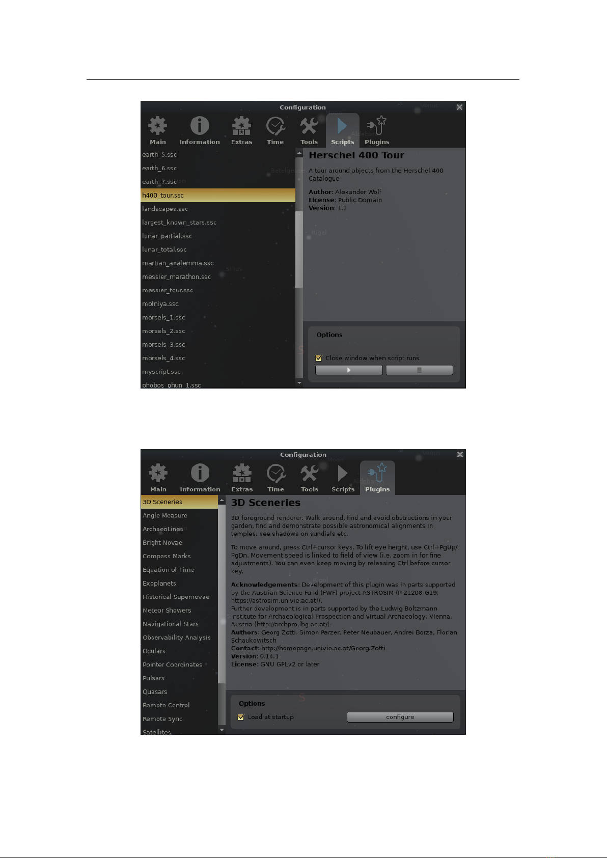
32 Chapter 4. The User Interface
equator, and the subsolar point (where the sun is at the zenith as seen from that feature). Features like
craters are best visible when they are illuminated by a low sun. You can therefore limit the display to
v 1.2
items along the terminator (the border between light and dark on the surface). You can also mark
v 23.3
craters and lunar maria (the dark “seas”) with circles.
GRS details. . .
: The Great Red Spot (GRS) is slowly drifting along Jupiter’s System II coordinate system.
This button opens a new dialog in which you can adjust the longitude (Jupiter system II) and annual
drift rate of this feature at a particular epoch. To help you, another button in this dialog opens a
website with relevant data. The central meridian data given in the object information on screen still
shows System II longitude.
Labels and markers
you can independently change the amount of labels displayed for Solar system objects.
The further to the right the sliders are set, the more labels you will see. Note that more labels will also
appear as you zoom in.
Planet magnitude algorithm
several ways to compute planet magnitudes have been made available from
the literature. Data by Müller (1893) provide visual magnitudes. The other models provide instrumen-
tal (Johnson V) magnitudes.
Earth shadow enlargement after Danjon
Earth’s shadow is enlarged by the atmosphere. You can select
whether the 2% enlargement used by the Astronomical Almanac should be applied (default), or the
formulation of DANJON (see section 19.11.2).
4.4.3 The Deep-Sky Objects (DSO) Tab
Deep-sky objects or DSO are extended objects which are external to the solar system, and are not point
sources like stars. DSO include galaxies, planetary nebulae and star clusters. These objects may or may
not have images associated with them. Stellarium comes with a catalog of over 90,000 extended objects
containing the combined data from many catalogs, with 500+ images.
The DSO tab (Fig. 4.13) allows you to specify which catalogs or which object types you are interested
in. This selection will also be respected in other parts of the program, most notably Search (section 4.5) and
AstroCalc/WUT (section 4.6.6) will not find objects from catalogs which you have not selected here.
See chapter 8 for details about the catalog, and how to extend it with your own photographs.
4.4.4 The Markings Tab
The Markings tab of the View window (Fig. 4.14) controls plotting various grids and lines on the celestial
sphere. Colors for grids, lines and points can be adjusted by clicking on the corresponding colored square.
The central column governs lines like equator, ecliptic, meridian etc., where each can optionally be fine-tuned
to show partition marks and labels. Color settings are stored immediately, all other flags need explicit saving
of the settings (see section 4.3.1).
4.4.5 The Landscape Tab
The Landscape tab of the View window (Fig. 4.15) controls the landscape graphics (the horizon which
surrounds you). To change the landscape graphics, select a landscape from the list on the left side of the
window. A description of the landscape will be shown on the right.
Note that while a landscape can include information about where the landscape graphics were taken
(planet, longitude, latitude and altitude), this location does not have to be the same as the location selected in
the Location window, although you can set up Stellarium such that selection of a new landscape will alter the
location for you.
The controls at the bottom right of the window operate as follows:
Use this landscape as default
Selecting this option will save the landscape into the program configuration
file so that the current landscape will be the one used when Stellarium starts.
Show ground This turns on and off landscape rendering (same as the button
in the main tool bar).
Show fog
This turns on and off rendering of a band of fog/haze along the horizon, when available in this
landscape.
Show illumination
to reflect the ugly developments of our civilisation, landscapes can be configured with a
layer of light pollution, e.g., streetlamps, bright windows, or the sky glow of a nearby city. This layer,
if present, will be mixed in when it is dark enough.
Show landscape labels
Landscapes can be configured with a gazetteer of interesting points, e.g., mountain
peaks, which can be labeled with this option. Color and font size can also be configured.
Location from landscape
When enabled, selecting a new landscape will automatically update the observer
location. Use this if the landscape is not just decoration, but a true representation of a particular site
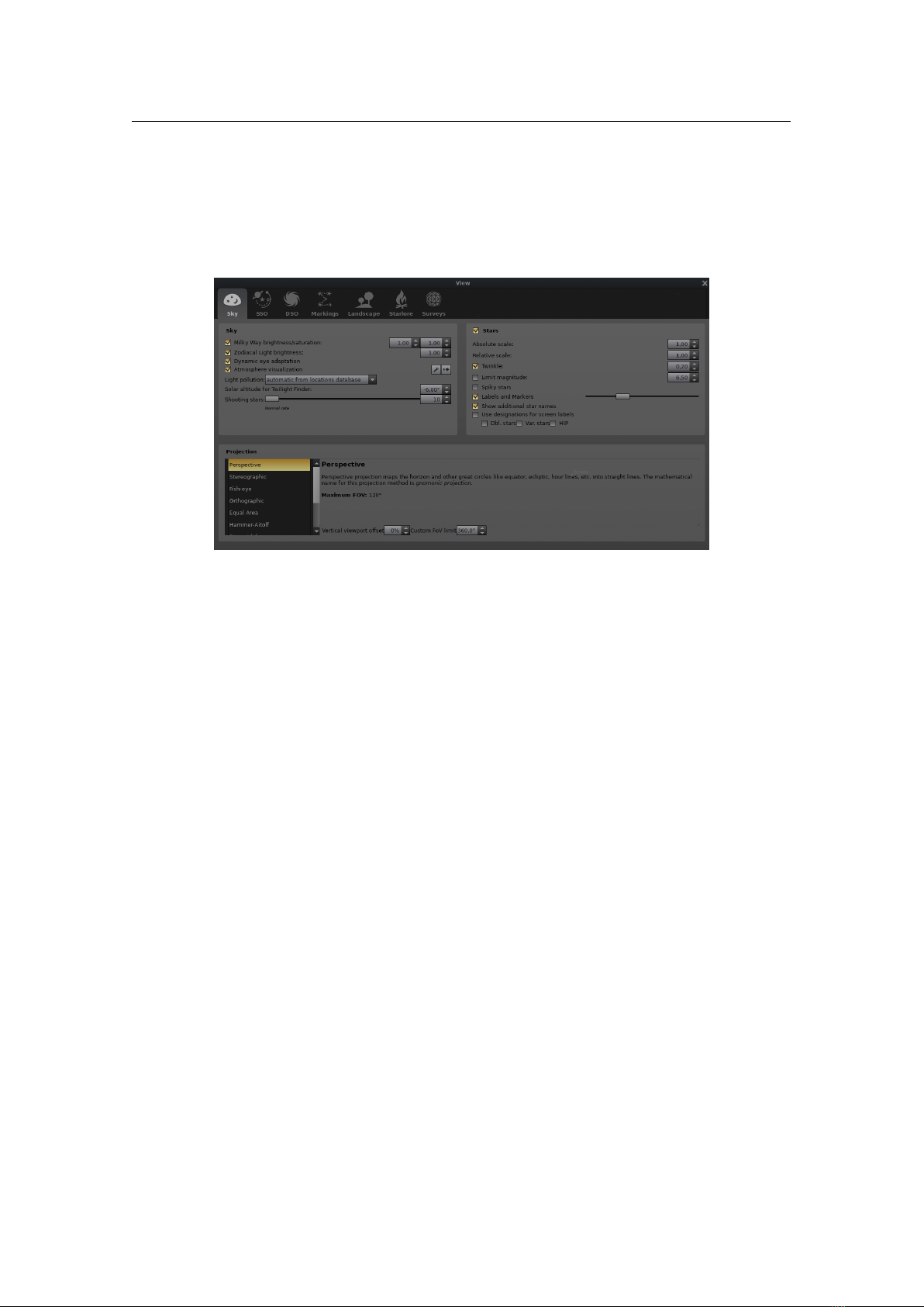
4.4 The View Settings Window 33
Figure 4.13: View Settings Window: DSO Tab
Figure 4.14: View Settings Window: Markings Tab
Figure 4.15: View Settings Window: Landscape Tab

34 Chapter 4. The User Interface
you wish to visit in the simulation.
Minimal brightness
Moonless night on very dark locations may appear too dark on your screen. You may
want to configure some minimal brightness here.
from landscape, if given
Landscape authors may decide to provide such a minimal brightness value
in the landscape.ini file.
Draw only polygon
If a polygonal horizon line has been defined for the landscape, only draw this with the
given thickness and color.
Transparency Allow peeking below the horizon. Note that this may show graphical errors.v 23.3
Using the button
Add/remove landscapes. . .
, you can also install new landscapes from ZIP files which you
can download e.g. from the Stellarium website
5
or create yourself (see ch. 7 Landscapes), or remove these
custom landscapes.
Loading large landscapes may take several seconds. If you like to switch rapidly between several
landscapes and have enough memory, you can increase the default cache size to keep more landscapes loaded
previously available in memory. Note that a large landscape can take up 200MB or more! See section D.1.13.
4.4.6 The Sky Culture Tab
Figure 4.16: World map showing Stellarium’s built-in set of sky cultures. To avoid overcrowding,
smaller European sky cultures which are mostly derivatives or relatives of the “Modern” sky culture
are not shown. (Image: S. M. Hoffmann)
If you want to explore humankind’s cultural history, you could also switch to the viewpoint of ancient or
other contemporary peoples. Constellations are defined as patterns in the sky shaped from fixed celestial
objects, often serving to set calendar marks and to navigate while travelling on Earth. Which patterns are
seen depends on the natural environment and the cultural habits of the people, i.e., the Inuit in the arctic
area might have seen an Elk where the Chinese have seen a huge spoon or dipper. There cannot be any
astrological influence from these patterns as they had been seen differently and, thus, are a product of
human’s imagination. So, pointing out these cultural differences might have an educational function, too.
Caution
Some of our native peoples’ constellations have been contributed for noncommercial use only. Please
respect their heritage holders and check-out the CC licence version in the description before you use sky
cultures for broadcasting! See section 9.1.3 for details.
The Sky Culture tab of the View window provides two sub-tabs:v 26.1
Details and Appearance
(Fig. 4.17) provides textual information about the currently selected skyculture,
and user interface elements to fine-tune the display of available data.
5
https://stellarium.org/landscapes.html
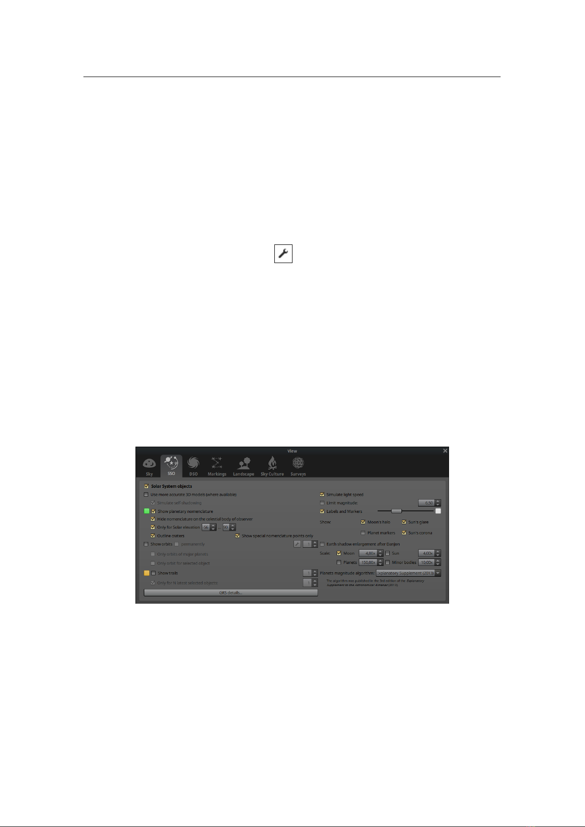
4.4 The View Settings Window 35
Figure 4.17: View Settings Window: Sky Culture Tab, Details and Appearance
Figure 4.18: View Settings Window: Sky Culture Tab, Exploration and Selection

36 Chapter 4. The User Interface
Exploration and Selection
(Fig. 4.18) provides a list of available skycultures, sorted into blocks of geo-
graphic regions, together with a world map on which the available cultures are displayed
6
. Clicking
on a polygon will select the respective skyculture.
On the tab “Details and Appearance”, you find numerous controls to configure how the current culture’s
constellations and bright star names will be used in the main display. Some cultures have constellation art
(e.g., Modern or Inuit), and the rest do not. Configurable options include
Use this sky culture as default Activate this option to load this sky culture when Stellarium starts.
Info and screen label styles
The new skyculture system has introduced a plethora of new name elements,
v 25.2
the complete set of which is not required to exist. There are name components that may come in
the skyculture’s original (native) language. If such a culture uses non-Latin glyphs in its writing,
non-native users need a transliteration that also helps pronunciation, which even depends on user
language. Then there are scientific transliteration systems for some cases. Finally, a pronunciation
aid can be given using the International Phonetic Alphabet (IPA). And, after the actual translation,
for reference, you may want to add the commonly used modern name to an object like star or planet.
There are two sets of settings, for the screen label and for the label used in the information area in the
top-left. The currently configured settings are immediately stored per-skyculture and retrieved when
you load another skyculture, so that you can adapt the system to your knowledge of languages and
character systems. See 9.2.9 for more.
Abbreviated names
To provide a less cluttered screen in case constellation names are long, you can
show abbreviations. The Modern skycultures use the 3-letter codes given by the IAU, for the other
skycultures we depend on our skyculture authors to define unique short labels that help memorizing.
Some skycultures still just show legacy numbers.
Select single constellation/Isolated See section 4.4.6.1 for details.
Constellation labels Activate display of constellation labels, like
or
V
.
Constellation lines
Activate display of stick figures, like or
C
, and you can configure constellation
line thickness in the right spinbox.
Constellation art
Activate display of constellation art (if available), like or
R
. You can also select
the brightness here.
Constellation boundaries
Activate display of constellation boundaries, like
B
. Currently, boundaries
have been defined only for “Modern” sky cultures.
Asterism labels Activate display of asterism labels, like
Alt
+
V
.
Asterism lines
Activate display of asterism stick figures (like the shortcut
Alt
+
A
), and you can configure
asterism line thickness as well.
Ray helpers
Activate display of special navigational lines which connect stars often from different constel-
lations (like the shortcut
Alt
+
R
), and you can configure thickness of those lines as well.
Constellation areas optional, advanced research feature. See page 119 for details.
Zodiac
If this skyculture has a concept of Zodiac (usually a region around the ecliptic split into 12 equal-
sized parts), you can enable it here.
Lunar Stations
If this skyculture has a concept of Lunar stations or mansions, you can enable them here.
For example, Indian skycultures observe 27 nakshatras along the ecliptic, and Chinese skycultures
have 28 Lunar mansions of unequal width in equatorial coordinates defined by particular stars.
4.4.6.1 Select single constellations
Some presenters may want to explain a particular storyline about the constellations of a sky culture, which
includes showing single constellations or showing a sequence of appearing constellations. To achieve this,
first activate “Select single constellation” mode (see fig 4.17). Then, click on a star which is part of a
constellation line set. Click another star which is part of another constellation to show that one in addition. If
you really only want to show a single constellation, also add the “Isolated” option.
If you explain a sky culture where constellations also have borders defined, a click anywhere in the
constellation area is enough. For other sky cultures, clicking onto a star which is not member of a constellation
line will display all constellations.
Press
W
to remove all but the last selected constellation. If you had deleted selection (right mouse
click) before pressing
W
, all constellations are hidden. Press
W
again to also hide the single displayed
one, or click another star to select the next constellation. If you need to keep the single constellation visible,
select the currently selected star again to select it again. Press
Alt
+
W
to show all constellations.
6
As of version 26.1 this is a new feature, and only Norse (Edda) so far has the polygons available.
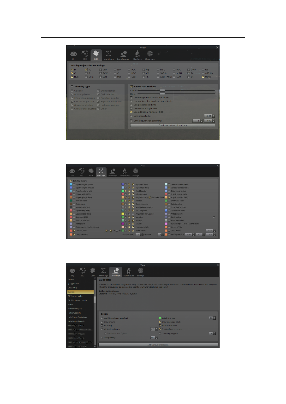
4.5 The Search Window 37
With a little training, you will be able to give inspiring constellation tours.
4.4.7 The Surveys Tab
Figure 4.19: View Settings Window: Surveys Tab
The Surveys tab (Fig. 4.19) allows to toggle the visibility of online sky or solar system surveys (see
chapter 10 for description of the surveys format). Currently, only HiPS surveys are supported.
On the left side of the window we see the list of available surveys from the configured sources (See
section D.1.30 for how to change the default sources). On the right side a description of the selected survey
and its properties are displayed.
Surveys are grouped by types. The top combobox allows to filter the listed surveys according to a given
type (Deep Sky or Solar System).
You can toggle the visibility of a survey by checking the box on the left of the survey name in the list.
(Note that as of v0.18.0, only a single deep sky survey can be rendered at a time, so it makes no sense to
select more than one in the list!) Once a survey is visible you should be able to see its loading status in the
loading bar area of the sky view.
Deep sky surveys will be rendered aligned with the sky view, while solar system surveys automatically
map on the proper body.
4.5 The Search Window
4.5.1 The Object tab
The Object tab of the Search window provides a convenient way to locate objects in the sky. Simply type in
the name of an object to find, and press . Stellarium will point you at that object in the sky.
As you type, Stellarium will make a list of objects which contains what you have typed so far. The first
of the list of matching objects will be highlighted. If you press the or key, the selection will change
to the next item in the list. Pressing the key will bring you to the previous item. Hitting the key will
center on the currently highlighted object and close the Search window.
For example, suppose we want to locate Saturn’s moon Mimas (SI). Open the Search window ( ,
F3
, or
Ctrl
+
F
). Type the first letter of the name, m, to see a list of objects whose name contains m:
Miranda (UV)
Psamathe (NX)
Umbriel (UII)
. . .
You may want at this point to have Stellarium rather propose object names which start with the string
you enter. Do that in the Options tab of this panel (see section 4.5.5). The search result should update
automatically when you navigate back to the Object tab. Now the list is shorter and contains only objects
which start with m:

38 Chapter 4. The User Interface
Figure 4.20: The Search Window: Object
Figure 4.21: The Search Window: Object (Recent Searches)
Figure 4.22: The Search Window: SIMBAD
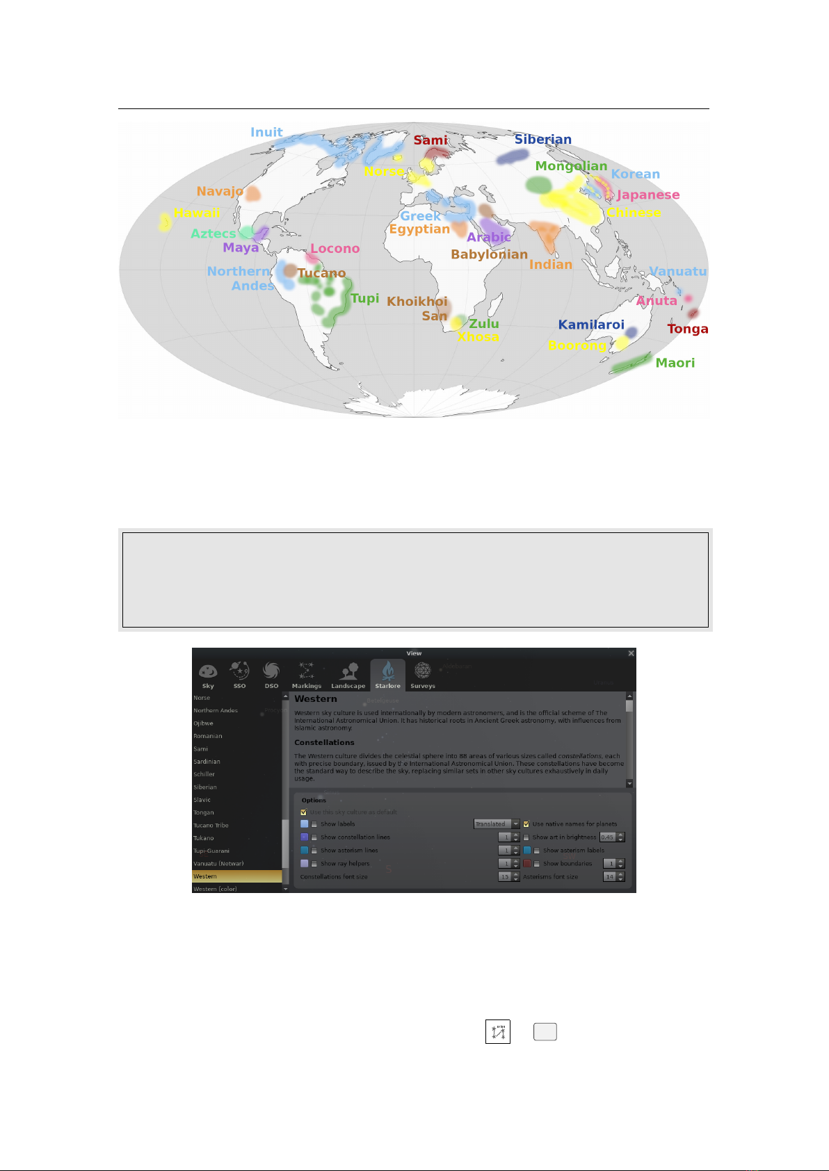
4.5 The Search Window 39
Figure 4.23: The Search Window: Position
Figure 4.24: The Search Window: Lists
Figure 4.25: The Search Window: Options
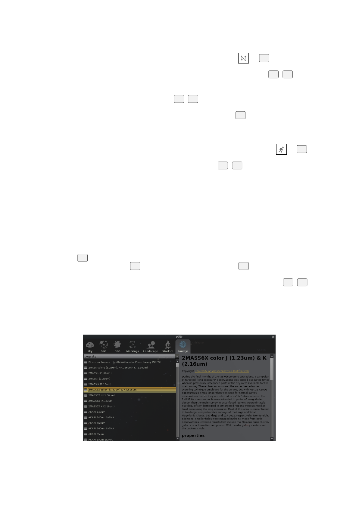
40 Chapter 4. The User Interface
Mago
Maia
Mars
. . .
The first item in this list, Mago, is highlighted. Pressing now would go to Mago, but we want Mimas
(SI). We can either press or a few times to highlight Mimas (SI) and then hit , or we can continue
to type the name until it is the first/only object in the list.
After you searched for an object, the next time the Search window opens, your most recently searched
object(s) will automatically appear in the search result of the Object tab. For instance, continuing with our
example, re-open the Search window’s Object tab. Mimas (SI) should already be populated and highlighted:
Mimas (SI)
The Object tab’s search result will now prioritize your most recent searches (which will be shown in bold).
To modify the search results, see section 4.5.5. From our earlier example, re-enter m into the Object tab.
Doing so will generate a slightly different list than before. In this case, Mimas (SI) will appear first, as shown
in Figure 4.21:
Mimas (SI)
Mago
Maia
Mars
. . .
4.5.2 The SIMBAD tab
The SIMBAD tab (Fig. 4.22) provides a convenient way to fetch and show a set of information for selected
object from the astronomical online database SIMBAD (Wenger et al., 2000). If some object is only visible
in a survey or DSS background (see section 10) and not in Stellarium’s catalogs, you can also set a custom
marker (see section 3.6), select it and query SIMBAD “tell me what’s known about objects at this location”.
4.5.3 The Position tab
The Position tab (Fig. 4.23) provides a convenient way to enter a set of coordinates.
4.5.4 The Lists tab
The Lists tab (Fig. 4.24) allows selection of an object from predefined sets. The number of choices is
governed by the loaded DSO catalogs and plug-ins. Scroll down the first window to select the type. Click on
the name and Stellarium will center on that object.
4.5.5 The Options tab
The Options tab (Fig. 4.25) provides a few settings to fine-tune your search experience.
Use SIMBAD
When the name of an object to find is typed in the Object tab and you are connected to the
internet and “Use SIMBAD” is ticked, Stellarium will search the SIMBAD on-line databases for its
coordinates. You can then click the button or press . Stellarium will point you at that object
in the sky even if there is no object displayed on the screen. The SIMBAD server being used can be
selected from the scroll window.
Server: for server selection
Search Options group allows for changes in the search result behaviour.
Use autofill only from the beginning of words
when checked, will search for object names that
begins with the same letters as your input. Example provided in section 4.5.1.
Lock position when coordinates are used
Show FOV center marker when position is search
Recent Searches
group allows modification to your recent search data. Any changes here will automatically
update the search results displayed in the Object tab. Example provided in section 4.5.1.
Max items to display amount of recent searches that can appear in the search result
button deletes your recent search history
4.6 The Astronomical Calculations Window 41
4.6 The Astronomical Calculations Window
This window provides advanced functionality, some of which is still under development. You can call it by
pressing
F10
or the button on the left menu bar. The Astronomical Calculations window shows eight
tabs with different functionality.
Most tabs allow exporting computed data to XLSX (Excel) files in addition to CSV files, and graphs
can be exported as PNG files.
4.6.1 The Positions Tab
This tab shows equatorial J2000.0 or horizontal positions, magnitudes and additional parameters (e.g. surface
brightness for deep-sky objects or angular separation for double stars) for various lists of celestial objects
above the horizon at the simulated time, filtered by magnitude. Double-clicking on an entry brings the object
into focus (Fig. 4.26). You may also export the list of positions into an XLSX or CSV file.
Figure 4.26: Astronomical Calculations (AstroCalc): Celestial positions / Seen now
This tab is split into 2 subtabs: “Seen now” and “Major planets”. The “Major planets” subtab (Fig. 4.27)
shows a table with heliocentric ecliptic positions of the major planets and a graphical representation of these
positions (in polar coordinates). You may also export the list of positions into an XLSX or CSV file.
Figure 4.27: Astronomical Calculations (AstroCalc): Celestial positions / Major Planets
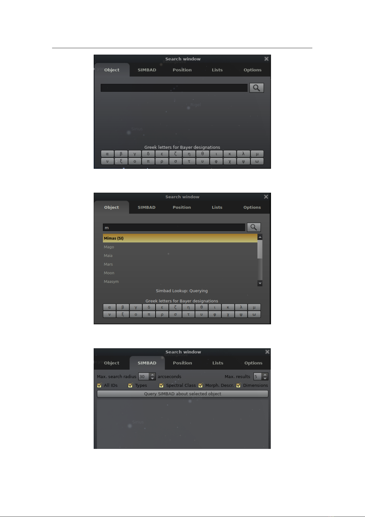
42 Chapter 4. The User Interface
4.6.2 The Ephemeris Tab
Select an object, start and end time, and compute an ephemeris (list of positions and magnitudes evolving
over time) for that object. The positions are marked in the sky with yellow disks (Fig. 4.28).
When you click on a date, an orange disk indicates this date and/or magnitude. Double-clicking sets the
respective date and brings the object to focus. Dates and/or magnitudes will show up near position markers
when Show dates and/or Show magnitudes checkboxes are active. To show a line between markers please
tick checkbox Show line. You may customize the format of displayed data near markers and their frequency
in the Extra options window (Fig. 4.29). You can also define the color of markers and enable display markers
for all naked-eye visible planets.
You can export the calculated ephemeris into an XLSX or CSV file.
Another interesting option in this tool: using horizontal coordinates for plotting traces of the Solar
system objects. In this mode, the circle marks are not linked to the sky, but to the horizontal coordinate
system. For example, you can get an analemma of the Sun for any location (Fig. 4.30 and 4.31), or observe
the visibility of Mercury, Venus or a comet in the twilight sky.
You can draw an ephemeris of two objects at the same time and define custom time step for the
ephemeris (Fig. 4.32).
Note: The ephemeris is computed with the current settings for atmosphere, topocentric correction etc. In
consequence, e.g. magnitudes may be affected by atmospheric absorption and may show unexpected values.
Remember to switch off atmosphere etc. to create extinction free geocentric mean positions as found in
almanachs.
Two time steps require a bit of care to display well. The Sun at preset altitude displays an object’s
v 26.2
position when the Sun is at a specific altitude relative to the horizon. Once selected from the list of time steps,
the Custom interval window is enabled, and a preset solar altitude can be selected (only values
≤ 0
○
are
valid), and the ephemeris is computed accordingly. If the Sun never reaches the altitude selected, during the
specified interval, e.g.
−12
○
during Scandinavian summer solstice, no marker is drawn. (Fig. 4.33). Using it
as intended requires the ephemeris to be drawn in horizontal coordinates!
The other time step that requires some care is the Opposition of planet. This is useful for displaying
where and when a planet will be at its opposition for a given year in relation to background stars. For it to
make sense, the planet in question needs to be selected both in the ephemeris list and in the Custom interval
window Fig. 4.34.
It is only applicable for the outer planets, i.e. Mars through Neptune. The computation is quite intense,
so showing e.g. Neptune oppositions throughout its 165 year orbit might take a while if you’re on a weak
system.
4.6.3 The “Risings, Transits, and Settings” (RTS) Tab
This tab allows you to compute meridian transits and rising and setting times of selected celestial object
(except unnamed stars and artificial satellites) for a specific date range. The tool is useful for planning
observations, and it suggests the best time and conditions for visual observations or astrophotography
(Fig. 4.35).
You may also export the list of transits into an XLSX or CSV file.
4.6.4 The Phenomena Tab
This tab allows you to compute phenomena like conjunctions, oppositions, occultations and eclipses (in
special cases) between planetary objects (Fig. 4.36). In addition, it provides computation of greatest
elongations for the inner planets and stationary points for all planets, and, for all Solar system bodies except
the moons, we also compute perihelia and aphelia.
You can export the calculated phenomena into an XLSX or CSV file.
Four columns in the table may be helpful for planning observation of phenomena:
solar elongation angular distance from the Sun
lunar elongation angular distance from the Moon
mag. 1 magnitude of first object
mag. 2 magnitude of second object
4.6.5 The Graphs Tab
This tab provides on several sub-tabs graphs which are helpful for monthly observation planning of deep-sky
objects and analysis of changes between objects or changes of their positions. Clicking in the graph sets the
time at that point, and setting the mouse onto a graph displays values at this point. However, most graphs are
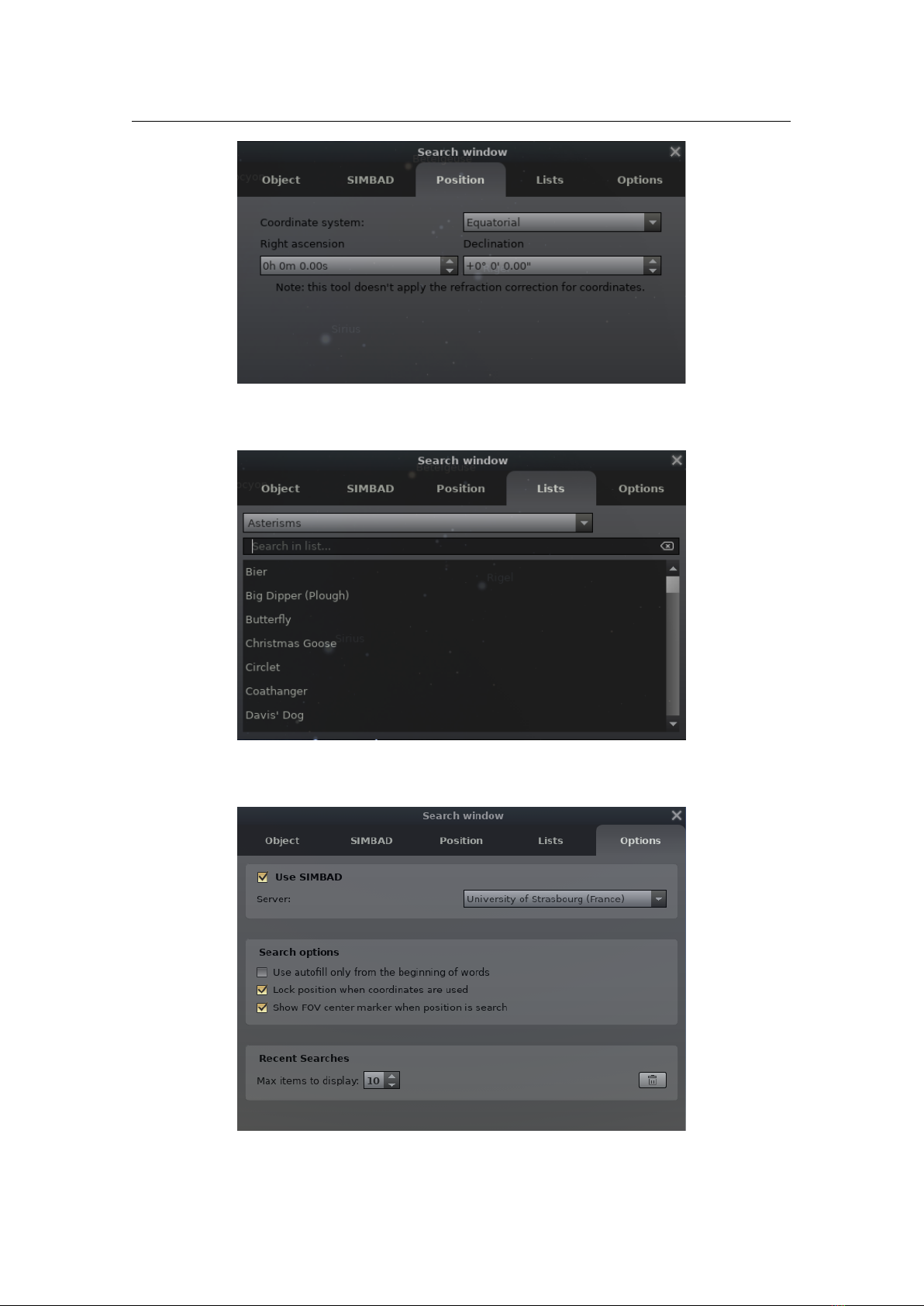
4.6 The Astronomical Calculations Window 43
Figure 4.28: Astronomical Calculations (AstroCalc): Plot trace of planet
Figure 4.29: Astronomical Calculations (AstroCalc): Extra options for ephemeris
Figure 4.30: Astronomical Calculations (AstroCalc): Analemma on the Earth

44 Chapter 4. The User Interface
Figure 4.31: Astronomical Calculations (AstroCalc): Analemma on Mars
Figure 4.32: Astronomical Calculations (AstroCalc): Two asteroids nearby to one place
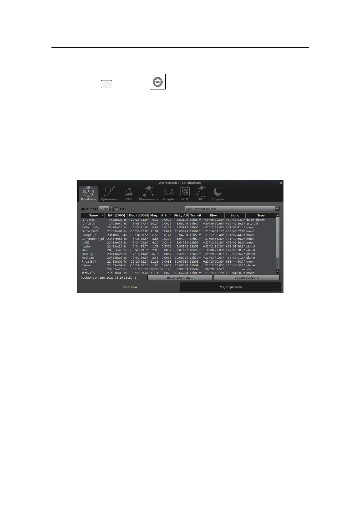
4.6 The Astronomical Calculations Window 45
Figure 4.33: Astronomical Calculations (AstroCalc): Venus when Sun is at the end of civil twilight
(-6°)
Figure 4.34: Astronomical Calculations (AstroCalc): Points of Saturn’s oppositions during a few
decades
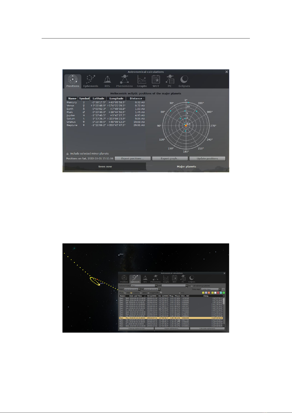
46 Chapter 4. The User Interface
Figure 4.35: Astronomical Calculations (AstroCalc): Risings, transits, and settings of selected
celestial object
Figure 4.36: Astronomical Calculations (AstroCalc): Phenomena
Figure 4.37: Astronomical Calculations (AstroCalc): Graphs / Altitude vs. Time
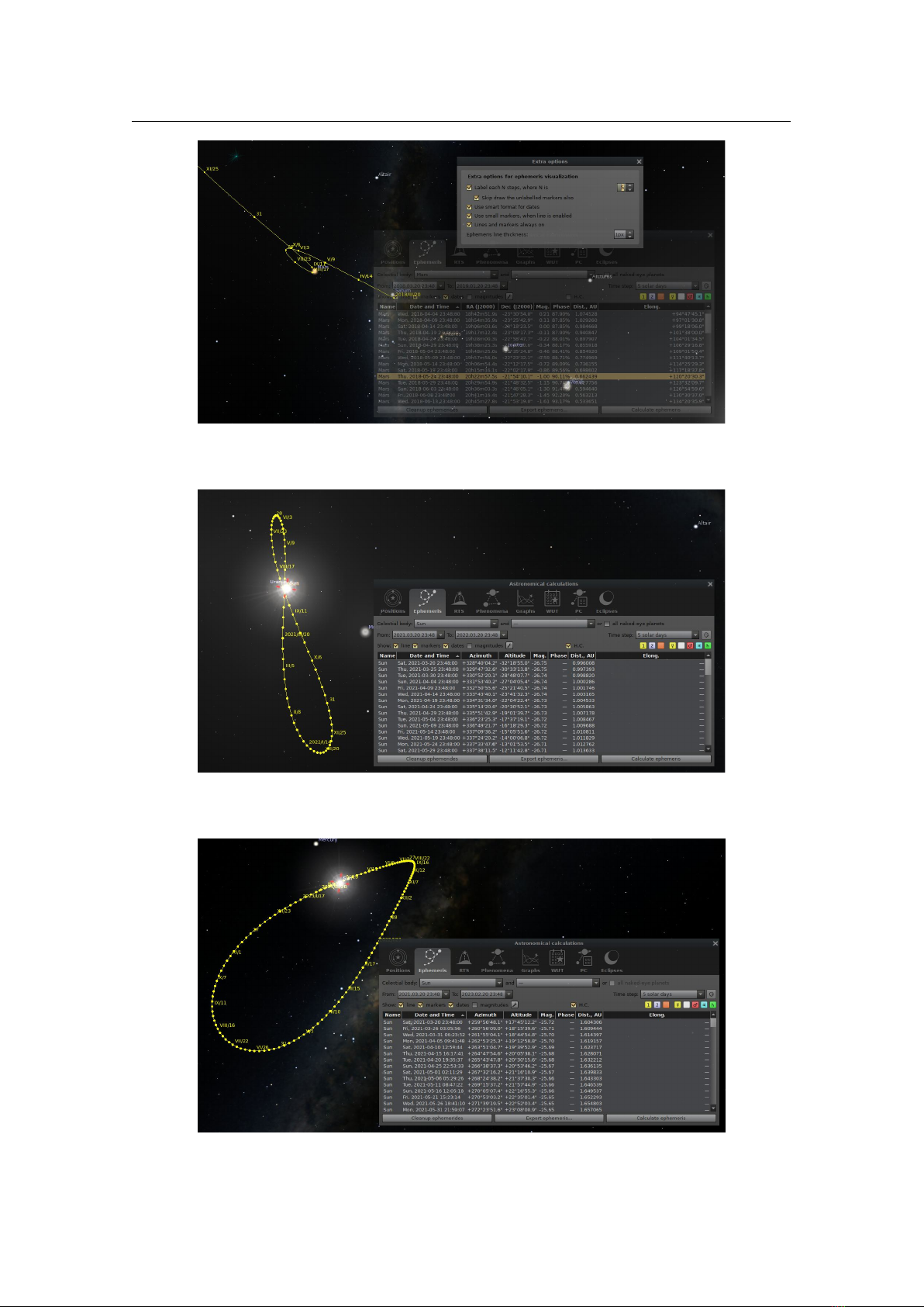
4.6 The Astronomical Calculations Window 47
Figure 4.38: Astronomical Calculations (AstroCalc): Graphs / Azimuth vs. Time
Figure 4.39: Astronomical Calculations (AstroCalc): Graphs / Monthly Elevation

48 Chapter 4. The User Interface
intended for a rapid overview and are plotted using an interpolating spline through sparse samples, so do not
expect highest accuracy.
4.6.5.1 The “Altitude vs. Time” Subtab
On this subtab (the first subtab and default view in the Graphs tab) you can compute the geometrical altitude
of the currently selected object on the currently set date and draw it as a graph (Fig. 4.37).
Optional graphs for the Sun (with lines for civil, nautical and astronomical twilight) and the Moon
(dashed) are also available.
4.6.5.2 The “Azimuth vs. Time” Subtab
On this subtab you can compute the geometrical azimuth of the currently selected object on the currently set
date and draw it as a graph (Fig. 4.38).
4.6.5.3 The “Monthly Elevation” Subtab
This subtab can show a “Monthly Elevation” graph for the current year at the selected time. This tool was
introduced for planning yearly observations (Fig. 4.39).
4.6.5.4 The “Graphs” Subtab
This subtab can show two functions over time for the current month or for up to 30 years and draw graphs
for them in one screen (Fig. 4.40). You can select from
•
Magnitude vs. Time
•
Phase vs. Time
•
Distance vs. Time
•
Elongation vs. Time
•
Angular size vs. Time
•
Phase angle vs. Time
•
Heliocentric distance vs. Time
•
Transit altitude vs. Time
•
Right ascension vs. Time
•
Declination vs. Time
This tool may be very helpful for educational and statistics purposes.
7
For example, the magnitude curve
for Jupiter’s moons shows occasional dips where the moon is in Jupiter’s shadow. However, while for most
graphs a sampling interval of 24 hours should be sufficient (i.e., 1 value per day), for this graph you may
want to reduce the sampling interval to 1 or 2 hours to avoid missing those eclipses by undersampling. Of
course, such high density takes much longer to compute, so you should avoid plotting this curve for many
years, or expect a long delay where the program may seem unresponsive.
4.6.5.5 The “Lunar Elongation” Subtab
This subtab (Fig. 4.41) can show a “Lunar Elongation” graph — the angular distance between the Moon and
the selected object (for example some deep-sky object) for the nearest 30 days. This tool was introduced for
planning monthly observations.
4.6.6 The “What’s Up Tonight” (WUT) Tab
The “What’s Up Tonight” (WUT) tool
8
displays a list of objects that will be visible at night for the current
date and location.
The objects are organized into type categories. Select an object type in the box labeled Select a Category,
and all objects of that type which are above the horizon on the selected night will be displayed in the box
labeled Matching Objects. For example, in the screenshot, the Planets category has been selected, and three
planets which are up in the selected night are displayed (Jupiter, Mars and Mercury).
By default, the WUT will display objects which are above the horizon between sunset and midnight (i.e.
in the evening). You can choose to show objects which are up between midnight and dawn (in the morning),
around midnight, or any time between dusk and dawn (any time tonight) using the combobox near the top
of the window. You can also choose to see only those objects that are brighter than a certain magnitude by
setting a minimum magnitude using the Show objects brighter than magnitude spinbox. You may center an
object from the right list in the sky map just by selecting it.
Note that only DSO from catalogs which you have selected in the DSO panel (section 4.4.3) will be
found.
In version 0.18.3 this tool has been refactored: the tool for searching items from list of Matching Objects
was removed, the filter for magnitudes was moved to the right, and we added a new filter here to limit the
7
The idea for this tool has been obtained from SkytechX: http://www.skytechx.eu/
8
This tool has been partially ported from the KStars planetarium: https://edu.kde.org/kstars/
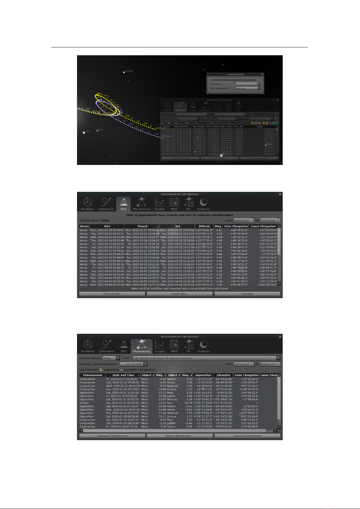
4.6 The Astronomical Calculations Window 49
Figure 4.40: Astronomical Calculations (AstroCalc): Graphs
Figure 4.41: Astronomical Calculations (AstroCalc): Graphs / Lunar Elongation
Figure 4.42: Astronomical Calculations (AstroCalc): What’s Up Tonight (WUT)
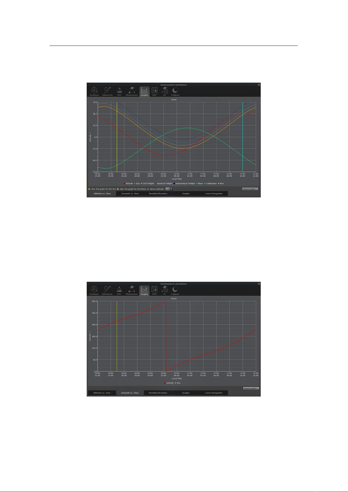
50 Chapter 4. The User Interface
Figure 4.43: Astronomical Calculations (AstroCalc): Planetary Calculator (PC), Data Tab
Figure 4.44: Astronomical Calculations (AstroCalc): Planetary Calculator (PC), Graphs Tab
Figure 4.45: Astronomical Calculations (AstroCalc): Eclipses / All Solar Eclipses
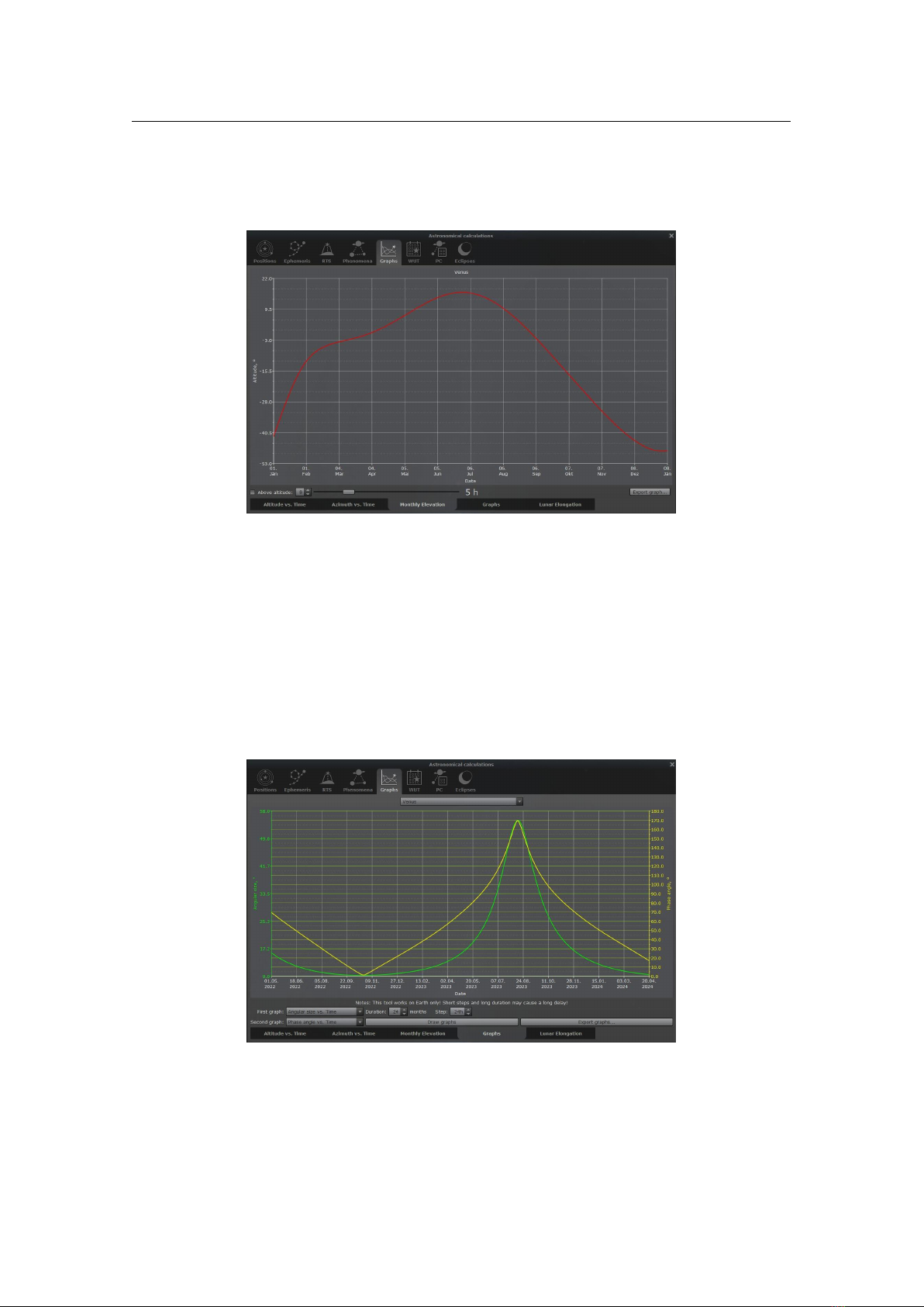
4.6 The Astronomical Calculations Window 51
range of acceptable angular sizes of matched objects. In addition to the names we added 5 new sortable
columns: magnitude, rising time, transit time, setting time and angular size of object.
4.6.7 The “Planetary Calculator” (PC) Tab
The “Planetary Calculator” (PC) tool has been added after user requests. It computes the relations between
two Solar system bodies for the current date and location — linear and angular distances, orbital resonances
and orbital velocities.
The Graphs tab (Fig. 4.44) shows the change in the linear and angular distances between selected
celestial bodies over a range of 600 days (centered on the current date) as graphs.
4.6.8 The Eclipses Tab
The Eclipses tool has four subtabs: “All Solar Eclipses”, “Local Solar Eclipses”, “Lunar Eclipses” and
“Planetary Transits”.
You can export the calculated eclipses and transits into an XLSX or CSV file.
Caution
Predicting eclipses and transits, and in particular local circumstances, over thousands of years in the past and
future is not reliable due to the principal unpredictability of
∆T
, caused by fluctuations of Earth’s rotation.
(See section 18.4.3 for details.)
4.6.8.1 The “All Solar Eclipses” Subtab
This subtab (Fig. 4.45) contains data for all solar eclipses on the Earth in the selected time range. Double
click on a line in the table will set location and time of greatest eclipse. Click on the table row will show
circumstances of selected eclipse in the lower table.
The quantity Gamma is the minimum distance of the lunar shadow cone axis to the center of the Earth,
in units of Earth’s equatorial radius. This distance is positive or negative, depending on whether the axis of
the shadow cone passes north or south of the Earth’s center.
Click the
Export KML. . .
button to create a KML file of the selected eclipse. KML is a file format used to
display geographic data in Earth browsers, such as Marble, Google Earth or Google Maps. The file can be
opened in applications that support KML version 2.2. A description of the lines for solar eclipses is shown
in Fig. 4.46. Different colors are used to draw path of central eclipse. Red = total eclipse, blue = annular
eclipse, and purple = hybrid eclipse. Limits of penumbral or partial eclipse are green.
4.6.8.2 The “Local Solar Eclipses” Subta b
This subtab (Fig. 4.47) contains data for solar eclipses for the current location (on the Earth!) in defined time
range.
Double click on a line in the table will set the time of greatest eclipse.
4.6.8.3 The “Lunar Eclipses” Subtab
This subtab (Fig. 4.48) contains data for all lunar eclipses on the Earth in defined time range. Double click
on the table row will set time of greatest eclipse. Click on the table row will show circumstances of selected
eclipse in the lower table.
The quantity gamma is the minimum distance from the center of the Moon to the axis of Earth’s umbral
shadow cone, in units of Earth’s equatorial radius. This distance is positive or negative, depending on whether
the Moon passes north or south of the shadow cone axis.
The visibility conditions are based on the altitude of the Moon at greatest eclipse:
Invisible — the greatest eclipse is invisible at the current location (altitude is negative);
Not obs.
— not observable eclipse. Our rule of thumb is that a partial penumbral eclipse is detectable with
the unaided eye if penumbral magnitude > 0.7;
Bad — bad visibility conditions for current location (altitude range is 0—30°);
Good
— good visibility conditions for current location (altitude range is 30—45°; i.e., “photometric
altitude”);
Perfect — perfect visibility conditions for current location (altitude range is 45—90°).
4.6.8.4 The “Planetary Transits” Subtab
This subtab (Fig. 4.49) contains data for all transits of Mercury and Venus across the Sun as seen from Earth
(see 19.11.3) in the defined time range. If an event is not observable because the Sun/planet is below the
horizon, its time will be shown in brackets and greyed-out. Further columns show the total duration of the
event, and the observable duration at the current location, which takes rising and setting times into account.
Double click on the table row will set time of mid-transit.

52 Chapter 4. The User Interface
Northern limit of penumbra (partial eclipse)
Total Solar Eclipse 2027 August 2
Southern limit of penumbra (partial eclipse)
Outline of umbra
plotted every 10 minutes
Point of greatest eclipse
Path of total eclipse
Southern limit
Northern limit
Center line
Eclipse begins at sunrise
Maximum eclipse at sunrise
Eclipse ends at sunrise
Eclipse begins at sunset
Maximum eclipse at sunset
Eclipse ends at sunset
Figure 4.46: Key to solar eclipse map
Figure 4.47: Astronomical Calculations (AstroCalc): Eclipses / Local Solar Eclipses
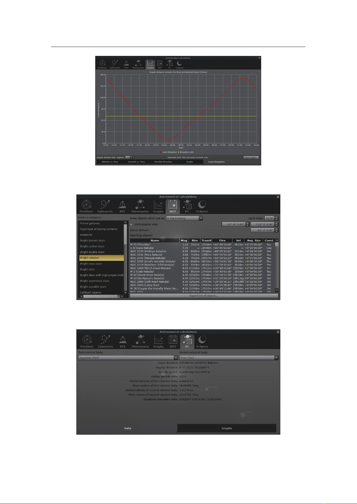
4.6 The Astronomical Calculations Window 53
Figure 4.48: Astronomical Calculations (AstroCalc): Eclipses / Lunar Eclipses
Figure 4.49: Astronomical Calculations (AstroCalc): Eclipses / Planetary Transits

54 Chapter 4. The User Interface
Figure 4.50: Astronomical Calculations (AstroCalc): Almanac / Specific Time
4.6.9 The Almanac Tab
The Almanac tool has one subtab: “Specific Time”.v 25.1
4.6.9.1 The “Specific Time” Subtab
This subtab (Fig. 4.50) contains data for specific time moments in this year (starring and duration seasons)
and at today — time for setting and rising the Sun and Moon, time and duration of twilights, and duration of
the daytime and astronomical night. You can use buttons to quick set these specific time moments. All dates
and times are selectable.

4.7 The Help Window 55
4.7 The Help Window
4.7.1 The Help Tab
Figure 4.51: Help Window
The Help Tab lists all of Stellarium’s keystrokes. Note that some features are only available as keystrokes, so
it’s a good idea to have a browse of the information in this window.
4.7.2 The About Tab
The About Tab (Fig. 4.52) shows version and licensing information, and a list of people who helped to
produce the program. This tab also provides a tool to check for updates of Stellarium.
4.7.3 The Log Tab
The Log Tab (Fig. 4.53) shows messages like the loading confirmations carried out when Stellarium runs. It
is useful to locate the files that Stellarium writes to your computer. The same information is written to the
file log.txt that you will find in your user data directory (see 5.1).
4.7.4 The Config Tab
The Config Tab (Fig. 4.54) shows configuration data of the Stellarium. It is useful to locate the files that
Stellarium writes to your computer. The same information is written to the file
config.ini
that you will
find in your user data directory (see 5.1).
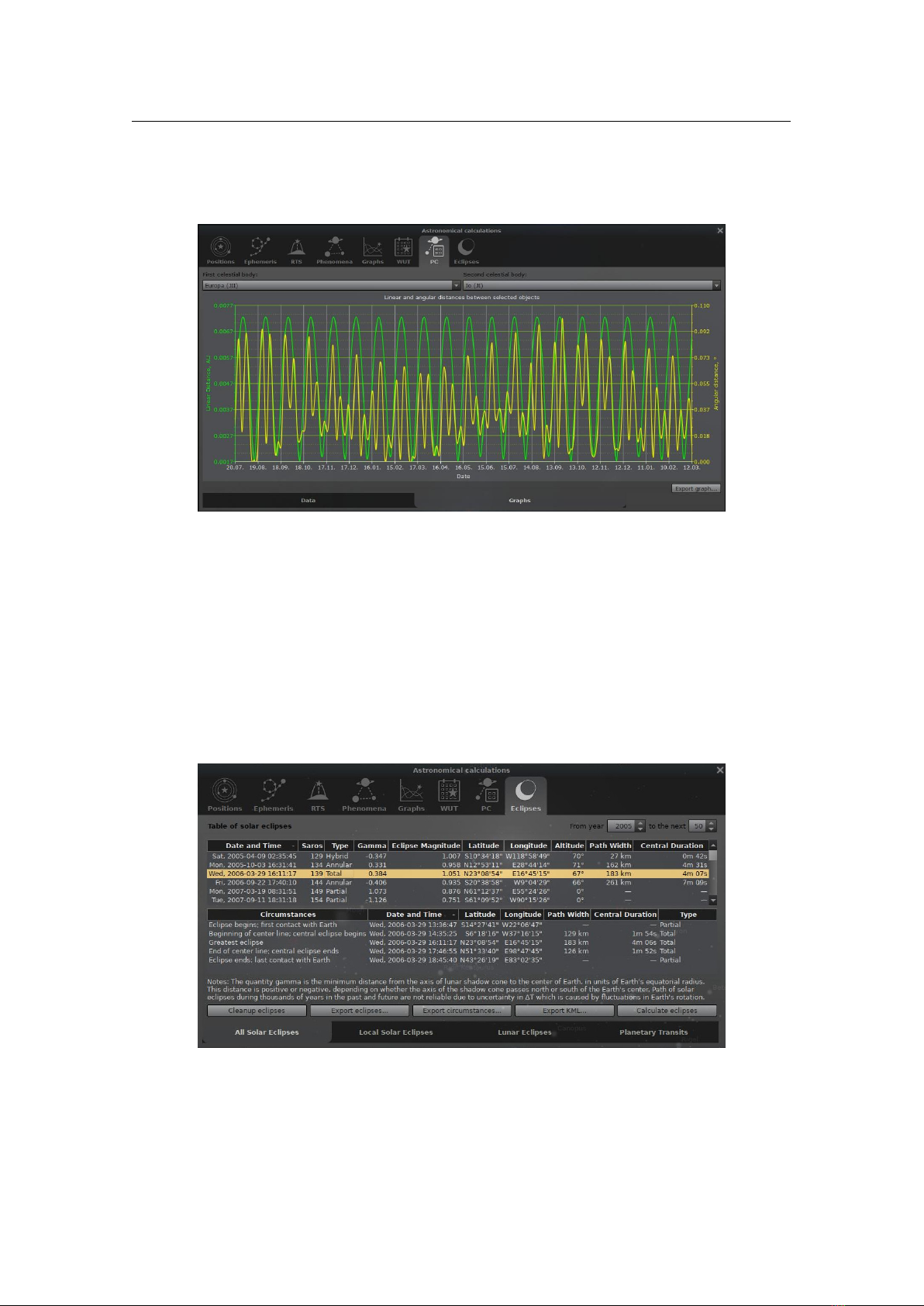
56 Chapter 4. The User Interface
Figure 4.52: Help Window: About
Figure 4.53: Help Window: Logfile
Figure 4.54: Help Window: Config file
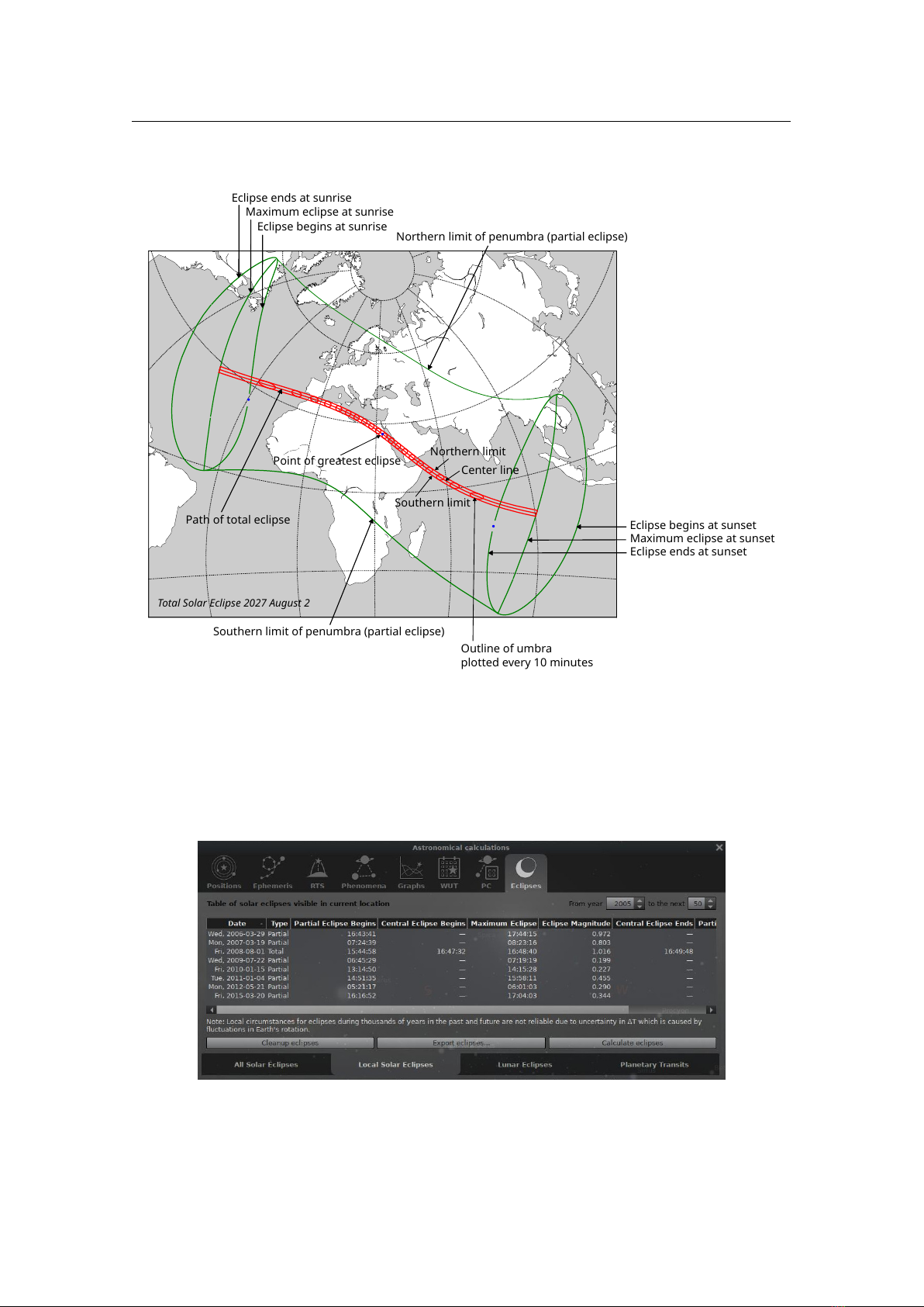
4.8 Editing Keyboard Shortcuts 57
4.8 Editing Keyboard Shortcuts
Figure 4.55: Keyboard Shortcuts
You can edit the shortcut keys here. Each available function can be configured with up to two key
combinations. You may want to reconfigure keys for example if you have a non-English keyboard layout and
some keys either do not work at all, or feel unintuitive for you, or if you are familiar with other software and
want to use the same hotkeys for similar functions. Simply select the function and click with the mouse into
the edit field, then press your key of choice. If the key has been taken already, a message will tell you.
This tool is available through the Help Tab of the Help window (see section 4.7.1) and the Tools Tab of
the Configuration window (see section 4.3.5).
4.8.1 Example
If you want to follow the sky view each evening with the Sun at the same depth below the horizon, so
that the twilight is of equal darkness, you may want to assign some actions to intuitive shortcut keys. In
the Keyboard Shortcut editor (Fig. 4.55), find the Date and Time group and assign, e.g., the keys on your
numeric keypad:
Previous evening twilight Ctrl+9
Previous morning twilight Ctrl+7
Next evening twilight Ctrl+3
Next morning twilight Ctrl+1
Today’s evening twilight Ctrl+6
Today’s morning twilight Ctrl+4
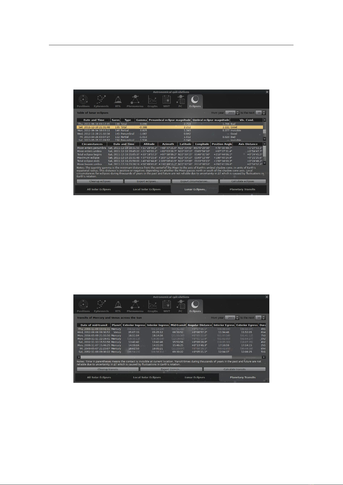
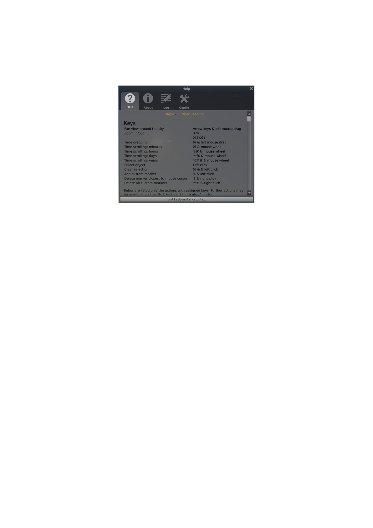
II
Advanced Use
5 Files and Directories . . . . . . . . . . . . . . . . . 61
5.1 Directories . . . . . . . . . . . . . . . . . . . . . . . . . . . . . 61
5.2 Directory Structure . . . . . . . . . . . . . . . . . . . . . . 62
5.3 The Logfile . . . . . . . . . . . . . . . . . . . . . . . . . . . . 63
5.4 The Main Configuration File . . . . . . . . . . . . . . . 63
5.5 Getting Extra Data . . . . . . . . . . . . . . . . . . . . . . 63
6 Advanced Options . . . . . . . . . . . . . . . . . . 67
6.1 Command Line Options . . . . . . . . . . . . . . . . . . 67
6.2 Environment Variables . . . . . . . . . . . . . . . . . . . 69
6.3 GUI Customizations . . . . . . . . . . . . . . . . . . . . . 70
6.4 Spout . . . . . . . . . . . . . . . . . . . . . . . . . . . . . . . . . 71
6.5 Show effects . . . . . . . . . . . . . . . . . . . . . . . . . . . 72
6.6 Spherical Mirror Mode for Planetarium Use . . . 72
7 Landscapes . . . . . . . . . . . . . . . . . . . . . . . . . 75
7.1 Stellarium Landscapes . . . . . . . . . . . . . . . . . . . 75
7.2 Creating Panorama Photographs for Stellarium 84
7.3 Panorama Postprocessing . . . . . . . . . . . . . . . . 89
7.4 Troubleshooting . . . . . . . . . . . . . . . . . . . . . . . . . 94
7.5 Other recommended software . . . . . . . . . . . . . 94
8 Deep-Sky Objects . . . . . . . . . . . . . . . . . . . 97
8.1 Stellarium DSO Catalog . . . . . . . . . . . . . . . . . . . 97
8.2 Adding Extra Nebula Images . . . . . . . . . . . . . . 103
9 Sky Cultures . . . . . . . . . . . . . . . . . . . . . . . . 109
9.1 Text description . . . . . . . . . . . . . . . . . . . . . . . . 109
9.2 Technical data: index.json . . . . . . . . . . . . . . . . 112
9.3 Territory description . . . . . . . . . . . . . . . . . . . . . 126
9.4 The Skyculture Converter . . . . . . . . . . . . . . . . . 126
9.5 Publish Your Work . . . . . . . . . . . . . . . . . . . . . . . 127
10 Surveys . . . . . . . . . . . . . . . . . . . . . . . . . . . . 129
10.1 Introduction . . . . . . . . . . . . . . . . . . . . . . . . . . . 129
10.2 Hipslist file and default surveys . . . . . . . . . . . . . 129
10.3 Solar system HiPS survey . . . . . . . . . . . . . . . . . . 130
10.4 Digitized Sky Survey 2 (TOAST Survey) . . . . . . . 130
11 Stellarium’s Skylight Models . . . . . . . . . 133
11.1 Introduction . . . . . . . . . . . . . . . . . . . . . . . . . . . 133
11.2 The Skylight Models . . . . . . . . . . . . . . . . . . . . . 133
11.3 Light Pollution . . . . . . . . . . . . . . . . . . . . . . . . . . 135
11.4 Tone Mapping . . . . . . . . . . . . . . . . . . . . . . . . . 135
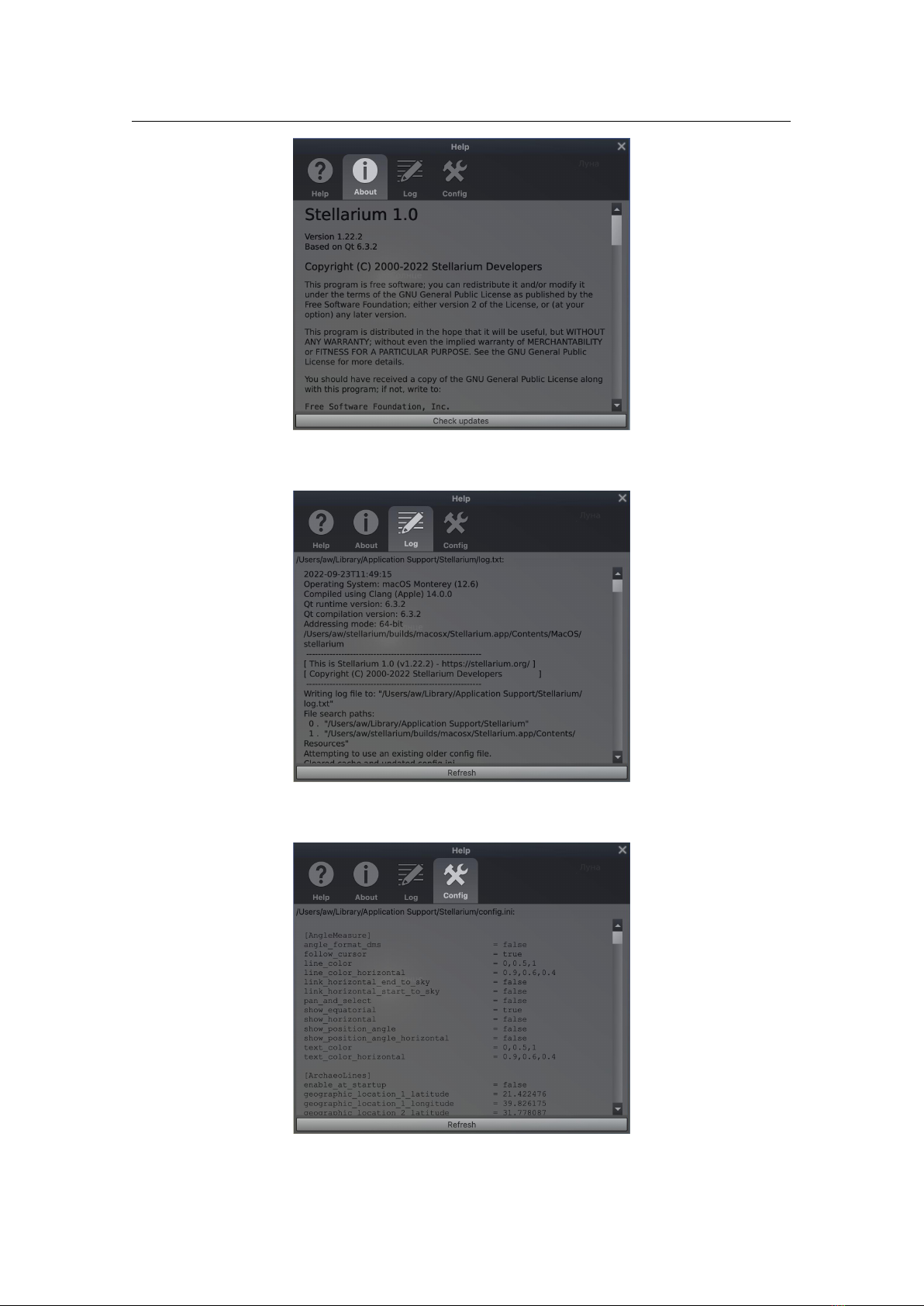
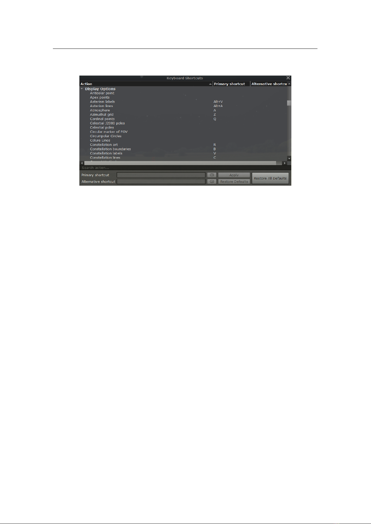
5. Files and Directories
5.1 Directories
Stellarium has many data files containing such things as star catalogue data, nebula images, button icons,
font files and configuration files. When Stellarium looks for a file, it looks in two places. First, it looks in
the user directory
1
for the account which is running Stellarium. If the file is not found there, Stellarium
looks in the installation directory
2
. Thus it is possible for Stellarium to be installed by an administrative user
and yet have a writable configuration file for non-administrative users. Another benefit of this method is on
multi-user systems: Stellarium can be installed by the administrator, and different users can maintain their
own configuration and other files in their personal user accounts.
In addition to the main search path, Stellarium saves some files in other locations, for example screens
shots and recorded scripts.
The locations of the user directory, installation directory, screenshot save directory and script save
directory vary according to the operating system and installation options used. The following sections
describe the locations for various operating systems.
5.1.1 Windows
installation directory
By default this is
C:\Program Files\Stellarium\
, although this can be adjusted
during the installation process.
user directory
This is the Stellarium sub-folder in the Application Data folder for the user account which is
used to run Stellarium. Depending on the version of Windows and its configuration, this could be any
of the following (each of these is tried, if it fails, the next in the list if tried).
% APPDATA %\ Stellarium \
% U SER PROF ILE %\ Ste lla rium \
% HOMEDRIVE %\% HOMEP ATH %\ S tel lar ium \
% HOME %\ Stellarium \
Stellarium ’s in stal lation dir ectory
Thus, on a typical Windows Vista/7/10 system with user “Bob Dobbs”, the user directory will be:
C :\ Users \ Bob Dobbs \ AppData \ Roa ming \ Ste lla rium \
The user data directory is unfortunately hidden by default. To make it accessible in the Windows file
explorer, open an Explorer window and select
Organize... Folder and search options
. Make sure
folders marked as hidden are now displayed. Also, deselect the checkbox to “hide known file name
endings”.
3
1
also called user data directory
2
The installation directory was referred to as the config root directory in previous versions of this guide
3
This is a very confusing default setting and in fact a security risk: Consider you receive an email with some file

62 Chapter 5. Files and Directories
screenshot save directory
Screenshots will be saved to the
Pictures/Stellarium
directory, although
this can be changed in the GUI (see section 4.3.5) or with a command line option (see section 6.1).
5.1.2 macOS
installation directory
This is found inside the application bundle,
Stellarium.app
. See The Anatomy of
macOS App Bundles
4
or Bundle Programming Guide
5
for more information.
user directory
This is the sub-directory
~/Library/Application Support/Stellarium
of the user’s
home directory.
screenshot save directory Screenshots are saved to the user’s Desktop.
5.1.3 Linux
installation directory
This is in the
share/stellarium
sub-directory of the installation prefix, i.e., usu-
ally /usr/share/stellarium.
user directory
This is the
.stellarium
sub-directory of user’s home directory, i.e.,
~/.stellarium/
.
This is a hidden folder, so if you are using a graphical file browser, you may want to change its settings
to “display hidden folders”.
screenshot save directory Screenshots are saved to the user’s home directory.
5.1.4 *BSD/Solaris/OpenIndiana
installation directory
This is in the
share/stellarium
sub-directory of the installation prefix, i.e., usu-
ally /usr/local/share/stellarium/.
user directory
This is the
.stellarium
sub-directory of user’s home directory, i.e.,
~/.stellarium/
.
This is a hidden folder, so if you are using a graphical file browser, you may want to change its settings
to “display hidden folders”.
screenshot save directory Screenshots are saved to the user’s home directory.
5.1.5 Haiku
installation directory This is in the /boot/system/data/stellarium/ sub-directory.
user directory
This is in the user’s home directory, i.e.,
~/config/settings/Stellarium/
or the sub-
directory /boot/home/config/settings/Stellarium/.
screenshot save directory Screenshots are saved to the user’s home directory.
5.1.6 Customized Location
Some users may prefer non-standard locations for their own data, for example when the Windows
C:
drive
(which usually contains user data), or the Linux
/home
partition has become too small to hold tens of
high-resolution landscapes or detailed 3D sceneries. You can move the entire directory elsewhere and use an
environment variable STEL_USERDIR that contains the pathname.
5.2 Directory Structure
Within the installation directory and user directory defined in section 5.1, files are arranged in the following
sub-directories.
landscapes/
contains data files and textures used for Stellarium’s various landscapes. Each landscape has
its own sub-directory. The name of this sub-directory is called the landscape ID, which is used to
specify the default landscape in the main configuration file, or in script commands.
skycultures/
contains constellations, common star names and constellation artwork for Stellarium’s
many sky cultures. Each culture has its own sub-directory in the skycultures directory.
scripts/ contains your own scripts. These can be used to create complex demonstrations (see ch. 17).
nebulae/
contains data and image files for nebula textures. In the future Stellarium may be able to support
multiple sets of nebula images and switch between them at runtime. This feature is not implemented
for version 26.3, although the directory structure is in place – each set of nebula textures has its own
sub-directory in the nebulae directory.
funny.png.exe
attached. Your explorer displays this as
funny.png
. You double-click it, expecting to open some
image browser with a funny image. However, you start some unknown program instead, and running this
.exe
executable
program may turn out to be anything but funny!
4
https://www.maketecheasier.com/anatomy-macos-app-bundles/
5
https://developer.apple.com/library/archive/documentation/CoreFoundation/Conceptual/CF
Bundles/Introduction/Introduction.html

5.3 The Logfile 63
stars/
contains Stellarium’s star catalogues. In the future Stellarium may be able to support multiple star
catalogues and switch between them at runtime. This feature is not implemented for version 26.3,
although the directory structure is in place – each star catalogue has its own sub-directory in the stars
directory.
data/ contains miscellaneous data files including fonts, solar system data, city locations, etc.
textures/
contains miscellaneous texture files, such as the graphics for the toolbar buttons, planet texture
maps, etc.
ephem/
(optional) may contain data files for planetary ephemerides DE430, DE431, DE440 and DE441
(see 5.5.3).
If any file exists in both the installation directory and user directory, the version in the user directory will
be used. Thus it is possible to override settings which are part of the main Stellarium installation by copying
the relevant file to the user area and modifying it there.
It is recommended to add new landscapes or sky cultures by creating the relevant files and directories
within the user directory, leaving the installation directory unchanged. In this manner different users on a
multi-user system can customise Stellarium without affecting the other users, and updating Stellarium will
not risk the loss of your own data.
5.3 The Logfile
Stellarium reports various events and confirmations to a logfile,
log.txt
, in the user directory. This has
the same content as you can see on the console on Linux when you start Stellarium on the command line.
Normally you don’t need to bother with its contents, however, if Stellarium behaves unexpectedly, crashes,
or shows other problems, a quick look into this file may help to identify the problem. Also when you report a
problem to the developers in the hope that they (we) can ’fix’ anything, this logfile is an essential ingredient
to your report. The logfile can also be displayed within the program: press
F1
to call the help panel, and
select the Logfile tab.
5.4 The Main Configuration File
The main configuration file is read each time Stellarium starts, and settings such as the observer’s location
and display preferences are taken from it. Ideally this mechanism should be totally transparent to the user
– anything that is configurable should be configured “in” the program GUI. However, at time of writing
Stellarium isn’t quite complete in this respect, despite improvements in each version. Some settings, esp.
color values for some lines, grids, etc. can only be changed by directly editing the configuration file.
6
This
section describes some of the settings a user may wish to modify in this way, and how to do it.
The name of the configuration file is
config.ini
7
. If the configuration file does not exist in the user
directory when Stellarium is started (e.g., the first time the user starts the program), one will be created with
default values for all settings (refer to section 5 Files and Directories for the location of the user directory on
your operating system).
The configuration file is a regular text file, so all you need to edit it is a text editor like Notepad on
Windows, Text Edit on the Mac, or nano/vi/gedit/emacs/leafpad etc. on Linux.
A complete list of configuration file options and values may be found in appendix D.1.
5.5 Getting Extra Data
5.5.1 More Stars
Stellarium is packaged with over 600 thousand stars in the normal program download, but much larger star
catalogues may be downloaded in the Tools tab of the Configuration dialog (
or
F2
).
6
Color values can be edited interactively by the Text User Interface plugin (see 13.6).
7
It is possible to specify a different name for the main configuration file using the
--config-file
command line
option. See section 6.1 Command Line Options for details.

64 Chapter 5. Files and Directories
5.5.2 More Deep-Sky Objects
Stellarium is packaged with over 94 thousand deep-sky objects
8
in the normal program download (the
standard edition of Stellarium DSO catalog
9
, see section 8.1), but an extended edition of DSO catalog with
over one million objects (up to
20.0
m
for galaxies) may be downloaded from Stellarium’s Github website
10
:
Version; Edition Filename MD5 hash Size
3.23; extended catalog-3.23.dat 56dfcdcedc3bfc18ce730984ab039308 28MB
The file can be placed in a folder named nebulae/default inside the user directory (see section 5.2).
5.5.3 Alternative Planet Ephemerides: DE430, DE431, DE440, DE441
By default, Stellarium uses the VSOP87 planetary theory, an analytical solution which is able to deliver
planetary positions for any input date (P. Bretagnon and Francou, 1988). However, its use is recommended
only for the year range
−4000. . . + 8000
. Outside this range, it seems to be usable for a few more millennia
without too great errors, but with degrading accuracy. Likewise for the moon, Stellarium by default uses
ELP 2000-82B (Chapront-Touze, 1982; Chapront-Touzé and Chapront, 1983; Chapront-Touzé and Chapront,
1988b).
Since v0.15.0 you can install extra data files which allow access to the numerical integration runs DE430
and DE431 (Folkner et al., 2014), and meanwhile also DE440 and DE441 (Park et al., 2021), from NASA’s
Jet Propulsion Laboratory (JPL). The data files have to be downloaded separately, and most users will likely
not need them. DE430 and DE440 provide highly accurate data for the years
+1550. . . + 2650
, while DE431
and DE441 covers years
−13000. . . + 17000
, which allows e.g. archaeoastronomical research on Mesolithic
landscapes. (But see Appendix F!) Outside these year ranges, positional computation falls back to VSOP87.
Some current approximations may still lead to numerical data which differ slightly from best possible
ephemerides. Please at least compare with JPL Horizons
11
for dependable results.
To enable use of these data, download the files from JPL
12
:
Ephemeris Filename MD5 hash Size
DE430 linux_p1550p2650.430 707c4262533d52d59abaaaa5e69c5738 97.5 MB
DE431 lnxm13000p17000.431 fad0f432ae18c330f9e14915fbf8960a 2.59 GB
DE440 linux_p1550p2650.440 9dc8a9cefd32b0090002407847e718ba 97.5 MB
DE441 linux_m13000p17000.441 4e3b924463d17b68ec9c4a18240300cd 2.59 GB
The files can be placed in a folder named
ephem
inside either the installation directory or the user
directory (see 5.2). Alternatively, if you have them already stored elsewhere, you may add the path to
config.ini like:
[ astro ]
de430_path = C :/ As trodata / JPL_DE43x / linu x_p15 50p26 50 .430
de431_path = C :/ As trodata / JPL_DE43x / lnxm 13000p17 000 .431
de440_path = C :/ As trodata / JPL_DE44x / linu x_p15 50p26 50 .440
de441_path = C :/ As trodata / JPL_DE44x / linu x_m1300 0p170 00 .441
For fast access avoid storing them on a network drive or USB pendrive!
You activate use of either ephemeris in the Configuration panel (
F2
). If you activate more than one,
preference will be given for DE440 over DE441 if the simulation time allows it. Only if DE44x are not
enabled, DE430 is given preference over DE431 if simulation time allows it. Outside of the valid times,
VSOP87 will always be used.
Acknowledgement
The optional use of DE430/431 has been supported by the ESA Summer of Code in Space 2015 initiative.
8
Over 83 thousand deep-sky objects in version 0.16.0.
9
The first number in the version of Stellarium DSO catalog means version of catalog structure, and the second
number means version of data.
10
https://github.com/Stellarium/stellarium-data/releases/tag/dso-3.23
11
https://ssd.jpl.nasa.gov/horizons.cgi
12
https://ssd.jpl.nasa.gov/ftp/eph/planets/Linux/
(Also download from this directory if you are not
running Linux!)
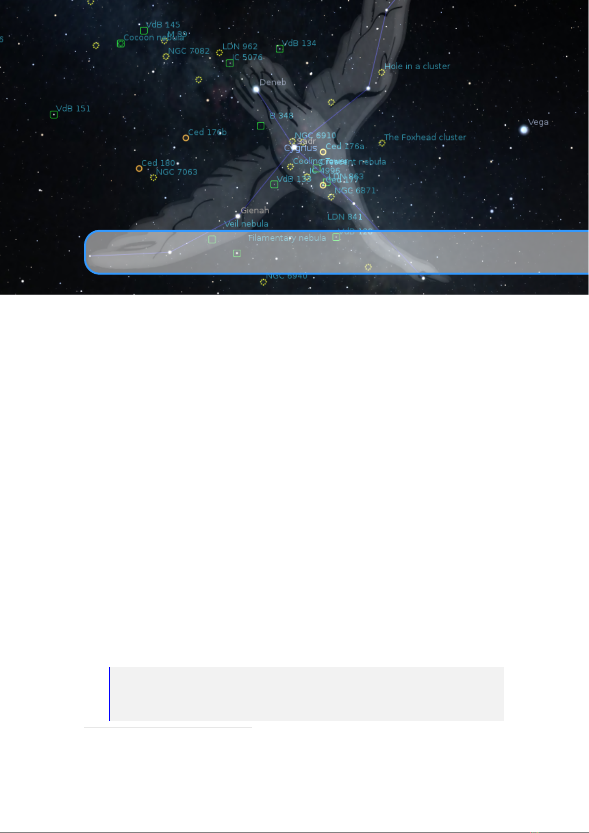
5.5 Getting Extra Data 65
5.5.4 GPS Position
In the Location panel (see section 4.2) you can receive your location from a GPS device. The exact way to
receive GPS location depends on your operating system.
5.5.4.1 GPSD (Linux, macOS only)
On Linux, Mac-OS X and other Unixoid platforms, Stellarium preferably should not connect directly to a
GPS USB device, serial device, bluetooth device, etc., but use a connection to the gpsd daemon running on
a computer in your network which provides GPS services concurrently for any interested application. In
most cases, this will be a gpsd running on your localhost, receiving data from some GPS device plugged in
via USB. Please follow instructions by the gpsd authors
13
to properly configure this system daemon. A few
hints:
•
On Ubuntu 16.04 and likely other systems, USB hotplug devices are handled by the udev daemon
which detects newly plugged-in devices and creates device files in the
/dev
directory. Unfortunately,
most GPS devices use the Prolific 2303 chipset in their serial-to-USB converter and are identified as
such, without other unique information like serial numbers. This chipset is also used in other Serial-
to-USB converter cables, and to avoid conflicts the according rule has been disabled by the release
managers of Ubuntu. In /lib/udev/60-gpsd.rules, find the commented line and re-activate it.
•
If you have such an USB GPS mouse and USB-to-serial converters for other purposes like for your
telescope control, you must solve the “udev crisis” in some other way to get gpsd running. You may
be able to find some property in your device to uniquely identify this device and write an udev rule to
create the symlink in /dev/gps0 to which gpsd can then connect.
•
You can also connect to another computer which runs gpsd. This could be a little Raspberry Pi
computer which happens to be in your WiFi to allow localisation and time service. To configure this,
you must manually edit config.ini. Find the [gui] section and edit
[ gui ]
# These values are used on non - Windows systems
# sup por tin g GPSD
gp sd_ hostn ame = lo cal host
gpsd_po rt = 2947
Also, gpsd must be started with the -G parameter to enable this.
•
Even your smartphone can be used as GPS data source
14
: Apps like BlueNMEA can provide these
data for gpsd, but you must make sure to configure hostname/IP Address and port number correctly,
for example
sudo gpsd -n -D8 -S 1001 tcp ://1 92 .168. 1. 101:435 2
which means
-n to start without a device connection
-D8 maximum debug level. When it works, use what suits you
-S 1001 provide service on port 1001
tcp
Use this address:port combination to receive data from (IP of your smartphone, port shown on
BlueNMEA screen).
•
In case you really don’t want to use the gpsd, you can use a directly connected device, see below.
This is however not recommended when you have gpsd available.
5.5.4.2 NMEA Device
This mode is primarily for Windows users, but also for Linux and Mac users who don’t want to use gpsd.
Virtually all GPS receivers are able to emit the standardized NMEA-0183 messages which encode time,
position, speed, satellite information and other data. The standard originally required connection settings of
4800 baud, 8 bit, no parity, one stop bit (8N1), however some devices come with faster transfer.
Compatible devices today are connected on a “virtual COM port” via USB. Unfortunately the COM
number seems to depend on the USB plug where you attach the receiver. You can identify the port name
(COM3, COM4, . . . ) in the Windows system configuration (Device Manager) or with the software that came
with your device.
15
13
https://gpsd.gitlab.io/gpsd/index.html
14
Thanks to user Caysho for this hint.
15
On Linux, this may read /dev/ttyUSB0, /dev/gps0 or similar.

66 Chapter 5. Files and Directories
If this is the only serial device, Stellarium should automatically connect to it regardless of configuration
entries. If you have a device with non-standard baudrate or several serial devices on serial ports (e.g., your
telescope?), you must find out which serial port is used by the GPS device and manually edit
config.ini
.
Find the [gui] section and edit
[ gui ]
# These values are used on Windo ws p rim arily .
gp s_i nterf ace = COM3
gps_b audr ate = 4800
From now on, always use the same USB plug configuration to connect GPS and telescope.
16
If GPS lookup fails, see section 6.2.1 to enable more diagnostic messages in the logfile.
Bluetooth GPS
Most smartphones provide GPS and Bluetooth hardware. You can install a virtual COM port in your
Windows Bluetooth settings and use a smartphone app like Share GPS
17
to provide the NMEA strings.
Windows location service
On Windows devices, you can get your location using the Windows location service. The result depends on
available hardware and other settings, e.g. real GPS sensor or network and WiFi detection.
18
5.5.5 Modernized MESA3D libraries (Software OpenGL on Windows)
Stellarium uses hardware-accelerated OpenGL for rendering. On very old Windows systems without
dedicated graphics hardware, or in special circumstances like virtual machines, hardware accelerated
graphics may not be available, and the Mesa3D software implementation of OpenGL is used. This can also
be forced by the command-line option
--mesa-mode
. Rendering the graphics without hardware acceleration
is of course much slower than accelerated graphics, but it’s surely better than nothing.
Qt’s default Mesa library (Mesa 11) provides support for OpenGL 3.0 only. This prevents users of all
versions from applying dithering in Mesa mode. Also the ShowMySky skylight model (see section 11.2.2) is
then not available.
We have replaced this by a version of Mesa 20 compiled by Federico Dossena
19
which appears to be
v 23.4
even a bit faster.
The Mesa3D project
20
meanwhile (2023) provides at least OpenGL 4.5. If you wish to use more “up to
date” precompiled binaries and have Administrator privileges on your Windows system, you can replace
this library using the following steps to install unofficial builds
21
. Note however that after this upgrade, the
program runs with considerably (
≈
35%?) lower framerate. You must decide whether this is really beneficial
in your situation. The libraries don’t provide any additional graphics features that Stellarium makes use of.
•
Download the latest “release-msvc” package as you need from
https://github.com/pal1000/m
esa-dist-win/releases and unpack it somewhere.
•
Copy
(x86|x64)/libglapi.dll,libgallium_wgl.dll,opengl32.dll
to where the executable
stellarium.exe is.
•
Delete the existing opengl32sw.dll
•
Rename the just-copied opengl32.dll to opengl32sw.dll.
Now running Stellarium in Mesa mode (with link from program menu or command line) should report to
provide OpenGL 4.5.
16
Again, for Linux the port number is defined in order of hotplugging by udev. You should develop an udev rule
which adds a unique name and use this. In this case, you may also need to add your user to the
dialout
group (or
whichever group owns your serial port). Better yet, use gpsd (see above).
17
https://play.google.com/store/apps/details?id=com.jillybunch.shareGPS
18
https://support.microsoft.com/en-us/windows/windows-location-service-and-privacy-3a8
eee0a-5b0b-dc07-eede-2a5ca1c49088
19
https://fdossena.com/?p=mesa/index.frag
20
https://www.mesa3d.org/
21
https://github.com/pal1000/mesa-dist-win/

6. Advanced Options
6.1 Command Line Options
Stellarium’s behaviour can be modified by providing parameters to the program when it is called via the
command line. See table for a full list:
Option Option Parameter Description
--help or -h [none]
Print a quick command line help message, and
exit.
--version or -v [none]
Print the program name and version information,
and exit.
--config-file or -c config file name
Specify the configuration file name. The default
value is config.ini.
The parameter can be a full path (which will be
used verbatim) or a partial path.
Partial paths will be searched for inside the reg-
ular search paths unless they start with a “
.
”,
which may be used to explicitly specify a file in
the current directory or similar.
For example, using the option
-c
my_config.ini
would resolve to the file
<user directory>/my_config.ini
whereas
-c ./my_config.ini
can be used to explicitly
point to the file
my_config.ini
in the current
working directory.
--log-file or -l
log file name
Specify the log file name. The default value is
log.txt.
The value of parameter can be a simple filename
or absolute path to the log file.
When a path is specified like
-l
my_log.txt
, the file will be written to
<user
directory>/my_log.txt
. When a path is spec-
ified like
-l /home/user/stellarium.log
/home/user/stellarium.log

68 Chapter 6. Advanced Options
--restore-defaults [none]
Stellarium will start with the default configura-
tion. Note: The old configuration file will be
overwritten.
--user-dir path Specify the user data directory.
--screenshot-dir
path
Specify the directory to which screenshots will
be saved.
--full-screen yes or no
Overrides the full screen setting in the config file.
--home-planet planet Specify observer planet (English name).
--latitude
latitude Specify latitude, e.g. 41.1 or +53d58’16.6"
1
--longitude
longitude Specify longitude, e.g. 16.2 or -1d4’27.48"
1
--altitude
altitude Specify observer altitude in meters.
--list-landscapes [none] Print a list of available landscape IDs and exit.
--landscape
landscape ID
Start using landscape whose ID matches the
passed parameter (dir name of landscape).
--sky-date date The initial date in yyyymmdd format.
--sky-time
time The initial time in hh:mm:ss format.
--startup-script script name
The name of a script to run after the program has
started. [startup.ssc]
--fov angle (degrees) The initial vertical field of view in degrees.
--scale-gui scale factor Scaling the GUI according to scale factor
--gui-css style
name Use name.css to define GUI style
--projection-type ptype The initial projection type: one of
ProjectionPerspective
ProjectionEqualArea
ProjectionStereographic
ProjectionFisheye
ProjectionCylinder
ProjectionCylinderFill
ProjectionMercator ProjectionMiller
ProjectionOrthographic
ProjectionHammer
ProjectionSinusoidal
--spout or -S all or sky Act as Spout sender (See section 6.4).
2,3
--spout-name
name
Use
name
as name of the Spout sender. Default
name: Stellarium.
2
--dump-opengl-details or -d [none]
Dump information about OpenGL support to log-
file. Use this is you have graphics problems and
want to send a bug report.
--angle-mode or -a [none]
Use ANGLE as OpenGL ES2 rendering engine
(autodetect Direct3D version).
2,4
--angle-d3d9 or -9
[none]
Force use Direct3D 9 for ANGLE OpenGL ES2
rendering engine.
2,4
--angle-d3d11
[none]
Force use Direct3D 11 for ANGLE OpenGL ES2
rendering engine.
2,4
--angle-warp
[none]
Force use the Direct3D 11 software rasterizer for
ANGLE OpenGL ES2 rendering engine.
2,4
1
You may have to escape the minute/second characters, like +53d58\’16.6\"
2
On Windows only
3
This function requires running in OpenGL mode.
4
Qt5-based Stellarium versions only

6.2 Environment Variables 69
--mesa-mode or -m [none]
Use MESA as software OpenGL rendering en-
gine.
2
--single-buffer
[none]
Use single-buffering. This reportedly avoids
screen blanking problems with some Intel GPUs.
--opengl-compat or -C [none]
Request OpenGL 3.3 Compatibility Profile.
Might fix graphics problems in some driver con-
figurations.
--low-graphics or -L
[none]
Force low-graphics mode. May be useful on old
GPUs that do support OpenGL 3.3 but perform
too slowly.
--no-audio [none]
Disable sound output (avoids initialisation prob-
lems on Virtual Machines or special builds).
--no-screensaver [none]
Disable screensaver and auto-sleep when in
fullscreen mode (Windows only).
If you want to avoid adding the same switch every time when you start Stellarium from the command line,
you can also set an environment variable STEL_OPTS with your default options.
Calling the respective options on the command line overrides settings from environment variables (apart
from STEL_OPTS).
6.1.1 Examples
•
To start Stellarium using the configuration file
configuration_one.ini
situated in the user direc-
tory (use either of these):
stellarium -- config - file = c onfig urati on_on e . ini
stellarium -c co nfigu ratio n_ one . ini
•
To list the available landscapes, and then start using the landscape with the ID “ocean”
stellarium -- list - landscapes
stellarium -- landsca pe = ocean
Note that console output (like --list-landscapes) may not be possible on some Windows systems.
6.2 Environment Variables
Some command-line options or settings can be set permanently by storing them into environment variables.
How to set them depends on the respective operating system.
Windows
Press the start menu, search for “environment variable”. Use the command to change user
variables. After setting, you can call Stellarium via its menu entry or desktop links.
This may be especially helpful on Windows systems with older graphics cards which may not
fully be compatible with OpenGL. Here we recommend you either use the program links using the
ANGLE-related options, or you can set the environment variable once and forget about the problems.
Linux, macOS
You will usually set such variables at the end of your
~/.bashrc
file. Open this with a text
editor and add, near the end,
export ST EL_OPTS ="- p latfo rm xcb -- single - buffer "
This forces use of the X11 platform plugin which may work better than wayland on older systems.
These environment variables are important:
STEL_OPTS
may contain a default commandline with options in the syntax of the table above. Also some
Qt settings can only be tweaked with this. For example, Windows users of international keyboards
with
Alt Gr
key may want to use
STE L _ O PTS =- pl a tform win d ows : altgr , fonte n g i n e = fr e e type -- single - bu ffer
The
-platform
parameter is part of Qt. Its second argument,
fontengine
, selects a different font
engine (i.e., some fonts may look better with it). The other argument,
- -single-buffer
, is a setting
that influences Stellarium (see table above).
STEL_USERDIR
may contain the path to a user data directory deviating from the default (see section 5.1).

70 Chapter 6. Advanced Options
QT_OPENGL
2
May be one of
desktop
(native OpenGL for your GPU, recommended),
angle
4
or
software
. The last activates pure software rendering using the MESA OpenGL library. Note that
command line options take precedence over this environment variable.
QT_ANGLE_PLATFORM
2,4
May be one of
d3d9
(DirectX 9) or
d3d11
(DirectX 11), or
warp
for
another software-only solution. Note that command line options take precedence over this environment
variable.
6.2.1 Logfile tweaks
Qt based programs can write log files where status messages of varying severity can be written
5
. There
are categories
debug
(usually only of developer interest),
info
(informational),
warning
(something unex-
pected),
critical
(usually connected to some real failure) and
fatal
(program fails (usually exits) here).
The amount of logging messages can be tuned by setting the environment variable
QT_LOGGING_RULES
. For
example, to remove all
debug
messages, set it to
*.debug=false;
. To remove even the
info
messages,
add
*.info=false;
. (Close each rule, also the last, with semicolon!) If you experience operating trouble,
make sure you allow all messages, i.e., set these entries shown here to true (or delete the variable).
Some modules can be individually finetuned with respect to the amount of logging. Most users won’t
v 25.4
ever want to see the ugly details, so debug is deactivated by default for:
stel.GPS GPS related issues.
stel.LocIP IP-based location queries.
stel.Texture Texture handling.
stel.Atmosphere Atmosphere related messages.
stel.Scripting scripting related messages.
stel.Media Multimedia related messages.
stel.HiPS HiPS related messages.
stel.Properties StelProperty related messages.
If you suspect issues with some features on your computer, add those entries as shown above, e.g., to
hunt down issues with a GPS device:
QT _LOGG ING_R ULES =*. debug = false ; stel . GPS . debug = true ;
or if you are developing scripts and videos don’t play, try if this helps:
QT _LOGG ING_R ULES =*. debug = false ; stel . Media . debug = true ;
6.3 GUI Customizations
Some users have difficulties to read Stellarium’s rather dark user interface. Some screens may be too dark, or
environments too bright.
6.3.1 Panel transparency
The GUI panels are semitransparent by design. If this impedes your ability to read them, you can make them
fully opaque with an entry to config.ini.
[ gui ]
fl ag _use_wind ow _transpar en cy = false
6.3.2 Button brightness
If you only want a bit brighter buttons, these can be tweaked separately in config.ini.v 24.4
[ gui ]
pi xmaps _b right ness =1.25
The value is clamped to [1. . . 1.8] to avoid making active and inactive buttons equally bright.

6.4 Spout 71
6.3.3 Text shadow
Some users complain the infotext is badly visible when there are trees or the Milky Way in the background.
v 24.4
This can also be mitigated in
config.ini
. The shadow (defaults shown) can be made slightly darker, but
not completely black. For additional darkness in screenshots at night, you can set a background opacity for
v 26.3
the info panel text. If you set this number negative, the dark background will be permanent, even in daylight,
using the color configured as “Overwrite text color” (s. 4.7).
[ gui ]
fl ag_in fo_sh adow = true
in fo_sh ad ow_ra dius =6 | [0...64]
in fo_shad ow_op acity =127 | [0 ...255]
in fo_pa ne l_opa city =0 | [ -100...100]
6.3.4 User interface color s
Others users still find the GUI too bright, and they would prefer a real “dark mode”. To allow this, you can
create and load your own alternative style files.
The appearance of the windows, buttons etc. is governed by a CSS (Cascaded Style Sheet) file. It
certainly requires some knowledge and guessing to edit your own, but there is enough general help on CSS
available online. You can find the CSS files in Stellarium’s Github site
6
.
Copy them into your user directory and rename to e.g.
myOwnGreatStyle.css
. Edit numbers, but do
not change the item names! Then you can either launch Stellarium with the added command line option like
stellarium -- gui - css myOwn Great Style
or you could also use the scripting option (see chapter 17):
core.setGuiStyle("MyOwnGreatStyle ");
To go back to Stellarium’s default, just use
core.setGuiStyle("default ");
If link colors in text panels are now difficult to read, copy
normalHtml.css
from Github to your own
MyOwnGreatStyleHtml.css and modify to your taste.
Note that, as Stellarium evolves, these files also may change from version to version. We cannot give any
guarantees that one customized file will work without adaptation on later or earlier versions of Stellarium.
6.4 Spout
Apart from stand-alone use, Stellarium can be used as multimedia source in larger installations, in museums
or science exhibitions. Spout
7
is a technology which enables use of Stellarium’s output window as texture in
DirectX applications on Windows. Simply start Stellarium with the
--spout=sky
command line option.
(Currently Spout output is limited to the main window without GUI panels, but this may change in future
versions.) Your master application must obviously embed a Spout receiver. The default name of the Spout
sender is
Stellarium
. If you need more than one instance of Stellarium acting as source, you can use
option
--spout-name=StelSpout2
in addition to create another Spout sender without a name conflict. In
such cases, it may be useful to also have separate user data directories and use option --user-dir.
This mode does not work in ANGLE mode and requires reasonably modern graphics hardware with the
WGL_NV_DX_interop
driver extension running in OpenGL mode. Some Nvidia GPUs work without this
extension listed explicitly. On a notebook with Nvidia Optimus technology, make sure to launch Stellarium
and SpoutReceiver (or your target application) on the Nvidia hardware. For permanent setting, use the
Nvidia configuration dialog to configure Stellarium and the target application explicitly to run always on the
Nvidia card.
Note that Spout use disables any multisampling setting (see Appendix D.1.26).
5
https://doc.qt.io/qt-6/qloggingcategory.html, https://doc.qt.io/qt-6/debug.html
6
https://github.com/Stellarium/stellarium/blob/stellarium-stable/data/gui/normalStyle.c
ss
and
https://github.com/Stellarium/stellarium/blob/stellarium-stable/data/gui/normalHtml.
css
7
https://spout.zeal.co/

72 Chapter 6. Advanced Options
6.5 Show effects
6.5.1 Sky Background
Stellarium is sometimes used for entertainment or artistic music performances. From this community a
request was placed to allow a non-black background. We can do that, but you must revert the color yourself.
Setting a background color is not available in the usual GUI to avoid inadvertent changes that later confuse
users. You can play with the sky background in the Text User Interface (see section 13.6.2, feature 5.26). In
config.ini, it is stored in
[ color ]
sk y_backg round_c olor = 0 .000000 ,0.000000 ,0 .000000
6.5.2 Star Trails
One of the oldest and previously simplest techniques from the time of film-based night photography is
v 26.2
the recording of Earth’s rotation by long-time exposure with an untracked camera. This will, for example,
identify the Polar Star as just not quite on the north celestial pole, but else show thousands of circular star
trails. While an exposure time of many hours is possible under dark skies, when the sky is too bright by
remaining twilight or light pollution, the exposure time meanwhile is often limited to minutes, else the
picture is just flooded with unwanted background.
Stellarium can be made to simulate such images by a somewhat “dirty trick”: Usually the image area is
cleared between frames, then the Milky Way, stars, Zodiacal light, grids, planets, atmosphere, landscape
etc., and finally GUI panels are rendered into the scene. By not clearing the image area, we can just add
up everything that is rendered on-screen, like in a long-time exposure. However, just as cars, airplanes,
satellites or people with flashlights can ruin your awesome star trail photo, some elements usually visible in
Stellarium’s sky would also create unwanted views. Image a celestial grid or the Milky Way rotating with the
sky, and twilight stacking all up and flooding the long-time exposure. The trick implemented in this special
mode draws one frame in “normal” mode, and then suppresses those elements and other details which cause
only smeared images like screen labels. A moderately long “exposure” can therefore still successfully show
constellations or star labels.
This is an option probably only used by instructors or presenters and therefore not preconfigured for
beginners. To make use of it, you must assign a keyboard shortcut to the action “Toggle star trails” found in
the “Display Options” key shortcut actions (see 4.8). While the mode is on, tapping
Ctrl
resets the trails. It
can make a nice ending scene in a presentation: show a moderately slow moving sky, and activate it. The
sky will fill with curves, hopefully impressing your audience. You can also utilize it when talking about the
problem of satellite constellations now destroying the sky. (Use realistic view, not icons, for satellites.) Here
your time speed should not be too fast, else satellites will just show up as dot chain.
Note that screenshots have to be made with system means while this mode is running.
6.6 Spherical Mirror Mode for Planetarium Use
IMMERSIVE-THEATRES.COM
With Stellarium it’s very easy to project the sky on a dome and create your own planetarium.
6.6.1 360° Projection
You can use either a very expensive fisheye lens projector – or a standard projector with a spherical mirror.
Not only is spherical mirror projection less expensive, but it produces a higher resolution image on the
dome
8
, and it’s very easy to upgrade the projector.
A planetarium spherical mirror is curved like a security mirror (convex safety mirror) – with the
important difference that its ‘first surface’, i.e., the reflective silver, is not protected by a transparent acrylic or
polycarbonate layer. This allows light to be reflected without being refracted. Spherical mirrors are therefore
very delicate and should never be touched with fingers or wiped with a cloth. A powerful dust blower is all
you need to keep it clean.
8
https://domeclub.com/#PxComp
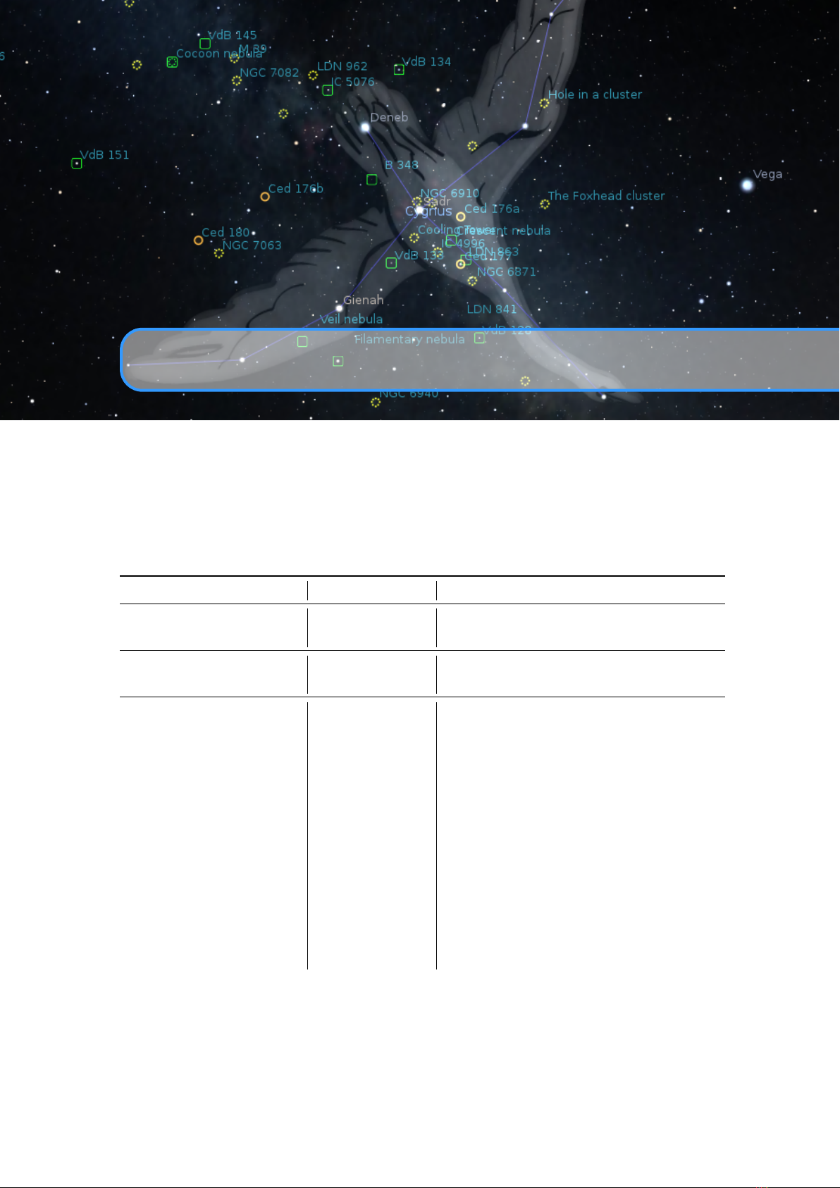
6.6 Spherical Mirror Mode for Planetarium Use 73
There are two types of spherical mirror projection boxes: compact ‘Newtonians’ (spherical mirror with
an additional small mirror)
9
; or full-length boxes (spherical mirror only)
10
. The former take up less space in
the planetarium (but a little less light reaches the dome); whereas the latter produce a slightly brighter image
(but require more space in the planetarium).
Although commercial projection boxes are quite expensive (mainly due to the cost of the first-surface
spherical mirror); it’s quite easy to build your own
11
– and you can use a cheap convex safety mirror for
testing before investing in a first-surface mirror.
6.6.2 Projector Specifications
A major challenge with digital planetariums (360° cinemas) is the cross-reflection of light on the dome. This
is why projector contrast ratio and colour saturation are more important than brightness (lumens). Light
‘bouncing’ around the dome causes the planetarium image to ‘wash out’ (lose colour) – so the higher the
projector colour saturation, the better. Similarly, the higher the contrast ratio, the sharper and crisper the
planetarium image will be, especially the night sky.
4K projectors are now very affordable, allowing you to deliver the same high-quality visuals in your
small dome as large planetariums!
6.6.3 Computer Configuration
The best way to operate a planetarium is with a dual display arrangement, i.e., computer screen as the primary
(main) display, and projector as the secondary (extended) display.
This way the Stellarium remote control window, desktop shortcuts, other applications, etc., will only be
visible to you. The audience will only see what you want them to see. To ensure there’s always something
nice on the dome (even with no application open), use a high-resolution image of stars as your desktop
wallpaper.
To function as a planetarium, Stellarium should be configured to open in full screen mode on the
extended display (see below).
6.6.4 System Configuration
To minimise image distortion at the back of the dome, it’s worth carrying out the slightly complex Meshmap-
per configuration
12
. This creates a custom distortion file for your specific system (i.e., your dome diameter,
stand height, spherical mirror dimensions); and the image improvement will be remarkable
13
. This custom
distortion file (‘warp mesh data file’) can then be used with dome applications like Stellarium.
6.6.5 Stellarium Configuration
To enable planetarium spherical mirror projection, the config.ini file needs to include the following:
[ navi gation ]
init _fov = 180
[ proj ection ]
type = Pr ojectio nFish eye
au to _z oom_out_r es ets_direc ti on = true
[ video ]
fullscreen = true
vi ewpor t_effect = sphe ri cMirr or Distort er
sc ree n_num ber = 1
[ s pheri c_mirror ]
di stort er_ma x_fov = 180
dome_ rad ius = 5.0 ( note : regardless of your actual dome radius )
im ag e_dista nc e_div_h ei ght = 2.67
mi rror_ posit ion_x = 0
mi rror_ posit ion_y = 5
mi rror_ posit ion_z = 0
9
https://www.eplanetarium.com/projector_newtonian.php
10
https://myplanetarium.com/projection-dome-system
11
https://docs.worldwidetelescope.org/diy-planetarium-dome/1/dome/#setting-up-the-proje
ctor-and-mirrors
12
https://paulbourke.net/dome/meshmapper
13
https://domeclub.com/images/Meshmapper-1152w.jpg

74 Chapter 6. Advanced Options
mi rro r_rad ius = 0.37 ( regardless of your actual mirror radius )
Stellarium also has built-in options to help you project the best possible planetarium night sky. In a
planetarium, removing the Stellarium atmosphere results in a much darker (and more beautiful) night sky.
Yet without the atmosphere, the stars stop twinkling and meteors (shooting stars) disappear – which is correct
for the real sky, but not what you may desire in the planetarium. To maintain twinkling and meteors even
without the atmosphere, manually add the following lines to the config.ini file:
[ stars ]
fl ag_forc ed_tw inkle = true
[ astro ]
fl ag _forced_m et eor_act iv ity = true
Another useful configuration for planetariums is to completely hide the vertical and horizontal toolbars
on the dome:
[ gui ]
fl ag_ show_ gui = false
The following are also recommended (adjust the values to your preference):
[ viewing ]
fl ag_mo on_sc aled = true
moon_scale = 8.00
[ astro ]
meteor_zhr = 3000
[ landscape ]
flag _fog = false
[ stars ]
ab solute_s cale = 6.00
fl ag_st ar_tw inkle = 1.00
fl ag_st ar_spiky = false
re lative_s cale = 0.70
st ar_twin kle_a mount = 0.50
6.6.6 Further notes
This feature is rarely used by the current developers and cannot be tested on standard hardware. See ongoing
discussion on Github
14
and get involved.
14
https://github.com/Stellarium/stellarium/issues/1914 and
https://github.com/Stellarium/stellarium/issues/3535
7. Landscapes
GEORG ZOTTI
Landscapes are one of the key features that make Stellarium popular. Originally just used for decoration,
since version 10.6 they can be configured accurately for research and demonstration in “skyscape astronomy”,
a term which describes the connection of landscape, the sky above, and the observer (D. Brown, 2015).
Configured properly, they can act as reliable proxies of the real landscapes, so that you can take e.g.
measurements of sunrise or stellar alignments (Zotti and Neubauer, 2015), or prepare your next moonrise
photograph, as though you were on-site.
In this chapter you can find relevant information required to accurately configure Stellarium landscapes,
using panoramas created from photographs taken on-site, optionally supported by horizon measurements
with a theodolite.
Creating an accurate panorama requires some experience with photography and image processing.
However, great open-source tools have been developed to help you on the job. If you already know other
tools, you should be able to easily transfer the presented concepts to those other tools.
While you are editing a landscape, you may want to reload it frequently. Turn off caching by editing the
config.ini:
[ landscape ]
ca che _size _mb = 0
7.1 Stellarium Landscapes
As of version 0.15, the available landscape types are:
polygonal
A point list of measured azimuth/altitude pairs, used to define a sharp horizon polygon. The area
below the horizon line is colored in a single color (Section 7.1.2).
spherical
The simple form to configure a photo-based panorama: A single image is used as texture map for
the horizon (Section 7.1.3).
old_style
The original photo panorama. This is the most difficult to configure, but allows highest resolution
by using several texture maps (Section 7.1.4).
fisheye
Another 1-texture approach, utilizing an image made with a fisheye lens. This landscape suffers
from calibration uncertainties and can only be recommended for decoration (Section 7.1.5).
A landscape consists of a
landscape.ini
plus the data files that are referenced from there, like a
coordinate list or the textures. Those reside in a subdirectory of the
landscape
folder inside the Stellarium
program directory, or, for own work, in a subdirectory of the
landscape
folder inside your Stellarium user
data directory (see section 5.1).

76 Chapter 7. Landscapes
Let us assume we want to create a landscape for a place called Rosenburg. The location for the files of
our new custom landscape Rosenburg depends on the operating system (see 5.1). Create a new subdirectory,
and for maximum compatibility, use small letters and no spaces:
Windows C:/Users/YOU/AppData/Roaming/Stellarium/landscapes/rosenburg
Linux ~/.stellarium/landscapes/rosenburg
Mac $HOME/Library/Application Support/Stellarium/landscapes/rosenburg
7.1.1 Location information
This optional section in
landscape.ini
allows automatic loading of site coordinates if this option is
activated in the program GUI (see 4.4.5). For our purposes we should consider especially the coordinates in
the location section mandatory!
[ location ]
planet = Earth
countr y = Austria
name = KGA Rosenburg
lati tude = +48 d38 ’ 3.3"
longitu de = +15 d38 ’2.8 "
alti tude = 266
time zone = Europe / Vienna
li ght_p ollution = 1
at mo sp he ric_extin ct io n_coefficie nt = 0.2
displ ay_ fog = 0
at mo spheric _temper at ure = 10.0
at mospher ic_pres sure = 1013.0
Where:
planet Is the English name of the solar system body for the landscape.
latitude
Is the latitude of site of the landscape in degrees, minutes and seconds. Positive values represent
North of the equator, negative values South of the equator.
longitude
Is the longitude of site of the landscape. Positive values represent East of the Greenwich
Meridian on Earth (or equivalent on other bodies), Negative values represent Western longitude.
altitude Is the altitude of the site of the landscape in meters.
country (optional) Name of the country the location is in.
state (optional) Name of the state the location is in.
timezone (optional) IANA Timezone code
name
(optional) Name of the location. This may contain spaces, but keep it short to have it fully visible in
the selection box.
Since v0.11.0, there are a few more optional parameters that can be loaded if the according switch is active
in the landscape selection panel. If they are missing, the parameters do not change to defaults.
light_pollution
(optional) Light pollution of the site, given on the Bortle Scale (1: none . . . 9: metropoli-
tan; see Appendix B). If negative or absent, no change will be made.
atmospheric_extinction_coefficient
(optional, no change if absent.) Extinction coefficient (mag/air-
mass) for this site.
atmospheric_temperature
(optional, no change if absent.) Surface air temperature (Degrees Celsius).
Used for refraction. Set to -1000 to explicitly declare “no change”.
atmospheric_pressure
(optional, no change if absent.) Surface air pressure (mbar; would be 1013 for
“normal” sea-level conditions). Used for refraction. Set to -2 to declare “no change”, or -1 to compute
from altitude.
display_fog
(optional, -1/0/1, default=-1) You may want to preconfigure setting 0 for a landscape on the
Moon. Set -1 to declare “no change”.
7.1.2 Polygonal landscape
This landscape type has been added to allow the use of measured horizons. Users of Cartes du Ciel
1
will be
happy to hear that the format of the list of measurements is mostly compatible.
1
SkyChart / Cartes du Ciel planetarium: https://www.ap-i.net/skychart/en/start

7.1 Stellarium Landscapes 77
This is the technically simplest of the landscapes, but may be used to describe accurately measured
horizon profiles. The file that encodes horizon altitudes can also be used in all other landscape types. If
present there, it will be used to define object visibility (instead of the opacity of the landscape photo textures)
and, if horizon_line_color is defined, will be plotted.
There are a few little caveats:
•
If you create a polygonal line with vertex azimuths 0, 90, 180, 270 (exactly), the horizon may not
show up at all. Add a tiny nonzero value to the global rotation, like
po ly gonal_a ngle_ro ta tez = 0.0000001
•
Sometimes, there may appear vertical lines from some corners towards the zenith or the mathematical
horizon, e.g. if there is a vertex including azimuth 0 or 180. If this irritates you, just offset this azimuth
minimally (e.g., 180.00001).
•
As technical requirement, the zenith is always assumed to remain free and uncovered. It is not possible
to define a “dome cutout” or similar restricted views out of a window. Such effect can be achieved
with a Spherical Landscape (see section 7.1.3).
The
landscape.ini
file for a polygonal type landscape looks like this (this example is based on the
Geneve landscape which was borrowed from Cartes du Ciel and comes with Stellarium):
[ landscape ]
name = Geneve
type = polygon al
author = Georg Zotti ; Horizon defi nit ion by Patrick Chevalle y
descr ipt ion = Hor izon line of Geneve .
Demon stra tes compati bility with
horizo n descrip tion s from Cartes du Ciel .
po ly gonal _h orizon_ list = hori zon_ Genev e . txt
po ly gonal_a ngle_ro ta tez = 0
groun d_co lor = .15 ,.45 ,.45
Where:
name appears in the landscape tab of the configuration window.
type identifies the method used for this landscape. polygonal in this case.
author lists the author(s) responsible for images and composition.
description
gives a short description visible in the selection panel. The text can be superseded by optional
description.<lang>.utf8 files.
polygonal_horizon_list is the name of the horizon data file for this landscape.
polygonal_horizon_list_mode
(optional) the two first columns in the list are numbers: azimuth and
altitude or zenith distance, in either degrees or radians or gradians(gon). The value must be one of
azDeg_altDeg
,
azDeg_zdDeg
,
azRad_altRad
,
azRad_zdRad
,
azGrad_altGrad
,
azGrad_zdGrad
.
Default: azDeg_altDeg
polygonal_angle_rotatez
(optional, default=0) Angle (degrees) to adjust azimuth. This may be used
to apply a (usually) small offset rotation, e.g. when you have measured the horizon in a grid-based
coordinate system like UTM and have to compensate for the meridian convergence.
ground_color
(optional, default=
0,0,0
, i.e., black) Color for the area below the horizon line. Each R,G,B
component is a float within 0..1.
minimal_brightness
(optional) Some minimum brightness to keep landscape visible. Default=-1, i.e.,
use minimal_brightness from the [landscape] section in the global config.ini.
minimal_altitude
(optional, default=-2) Some sky elements, e.g. stars, are not drawn below this altitude
to increase performance. Under certain circumstances you may want to specify something else here.
(since v0.14.0)
polygonal_horizon_inverted
(optional, default=false; only required in v0.15.0–0.20.2) In rare cases
like horizon lines for high mountain peaks with many negative horizon values this should be set to
true.
No longer used:
horizon_line_color
(optional, default: invisible) used to draw a polygonal horizon line. This is now a
v 24.4
global setting, config.ini:landscape/polygon_color.

78 Chapter 7. Landscapes
7.1.2.1 Artificial Polygonal Panoramas
The online service HeyWhatsThat
2
allows an SRTM-based analysis of the viewshed (the visible topographic
area) for an observing location which also gives names for the mountain peaks visible at a given location. In
summer of 2020 a dedicated landscape download option for Stellarium was added (see upper-right corner),
so that you can install a custom landscape. Its package/directory name is
stellarium-landscape
. If you
create more than one, you must rename the directory. You may also want to extend the scene description in
landscape.ini.
See section 7.3.4 for more options.
7.1.3 Spherical landscape
This method uses a more usual type of panorama – the kind which is produced directly from software such
as autostitch or Hugin
3
. The Moon landscape which comes with Stellarium provides a minimal example of
a landscape.ini file for a spherical type landscape:
[ landscape ]
name = Moon
type = spheric al
maptex = apol lo17 . png
A more elaborate example is found with the Grossmugl landscape:
[ landscape ]
name = Grossmu gl
type = spheric al
author = Guen ther Wuchterl , Kuffner - S ter nwa rte . at ;
Lightscape : Georg Zotti
descr ipt ion = Field near Leeberg , Gr ossmugl ( Ries entumulus ),
Austri a - Primary Obse rving Spot of the Grossmugl
Starlig ht Oasis - http :// starl ighto asis . org
maptex = gros sm ugl_lee be rg_crop 11 .25. png
maptex_top =11.25
maptex_fog = gr os sm ugl_lee be rg _fog_cr op 22 .5. png
ma ptex_fog _top = 22.5
ma ptex_ fog_b ottom = -22.5
mapte x_il lum = grossm ug l_ leeberg _i ll um_crop0 . png
ma ptex_il lum_b ottom = 0
an gle _rota tez = -89.1
mi nimal _b right ness = 0.0075
po ly gonal _h orizon_ list = hori zon_g ro ssmug l . txt
po ly gonal_a ngle_ro ta tez =0
mi nimal _alti tude = -1
Where:
name appears in the landscape tab of the configuration window. This name may be translated.
type identifies the method used for this landscape. spherical in this case.
author lists the author(s) responsible for images and composition.
description
gives a short description visible in the selection panel. The text will be superseded by
optional description.<lang>.utf8 files.
maptex is the name of the image file for this landscape.
maptex_top (optional; default=90) is the altitude angle of the top edge.
maptex_bottom
(optional; default=-90) is the altitude angle of the bottom edge. Usually you will not
require this, or else there will be a hole at your feet, unless you also specify
bottom_cap_color
(optional; default=
-1.0,0.0,0.0
to signal “no color”). If set, this is used to close
any hole in the nadir area (if maptex_bottom higher than -90).
maptex_fog (optional; default: no fog) is the name of the fog image file for this landscape.
2
https://www.heywhatsthat.com/
3
http://hugin.sourceforge.net/
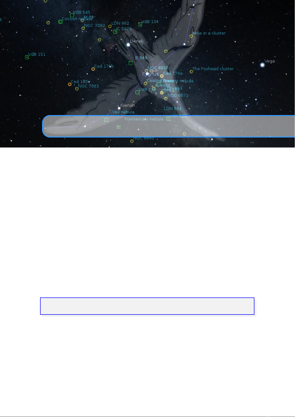
7.1 Stellarium Landscapes 79
maptex_fog_top
(optional; default=90) is the altitude angle of the top edge of the fog texture. Useful to
crop away parts of the image to conserve texture memory.
maptex_fog_bottom (optional; default=-90) is the altitude angle of the bottom edge.
maptex_illum
(optional; default: no illumination layer) is the name of the nocturnal illumination/light
pollution image file for this landscape.
maptex_illum_top
(optional; default=90) is the altitude angle of the top edge, if you have light pollution
only close to the horizon.
maptex_illum_bottom (optional; default=-90) is the altitude angle of the bottom edge.
angle_rotatez
(optional, default=0) Angle (degrees) to adjust azimuth. If 0, the left/right edge is due
east.
tesselate_rows
(optional, default=20) This is the number of rows for the maptex. If straight vertical
edges in your landscape appear broken, try increasing this value, but higher values require more
computing power. Fog and illumination textures will have a similar vertical resolution.
tesselate_cols
(optional, default=40) If straight horizontal edges in your landscape appear broken, try
increasing.
polygonal_horizon_list
(optional) is the name of the (measured) horizon data file for this landscape.
Can be used to define the exact position of the horizon. If missing, the texture can be queried for
horizon transparency (for accurate object rising/setting times)
polygonal_horizon_list_mode (optional) see 7.1.2
polygonal_angle_rotatez (optional, default=0) see 7.1.2
minimal_brightness see 7.1.2
minimal_altitude
(optional, default=-2) Some sky elements, e.g. stars, are not drawn below this altitude
for efficiency. Under certain circumstances (e.g. for space station panoramas where you may have sky
below your feet, or for deep valleys/high mountains, you may want to specify something else here.
To save texture memory, you can trim away the transparent sky and define the angle
maptex_top
. Like-
wise,
fogtex_top
,
fogtex_bottom
,
maptex_illum_top
and
maptex_illum_bottom
. You should then
stretch the texture to a full power of 2 for maximum compatibility, like
4096× 1024
(but note that some
hardware is even limited to 2048 pixels). The easiest method to create perfectly aligned fog and illumination
layers is with an image editor that supports layers like the GIMP or Photoshop. Fog and Light images should
have black background.
7.1.4 High resolution (“Old Style”) landscape
The
old_style
or multiple image method works by having the 360°panorama of the horizon (without
wasting too much texture memory with the sky) split into a number of reasonably small side textures, and a
separate ground texture. This has the advantage over the single-image method that the detail level of the
horizon can be increased without ending up with a single very large image file, so this is usable for either
very high-resolution panoramas or for older hardware with limited capabilities. The ground texture can be a
different resolution than the side textures. Memory usage may be more efficient because there are no unused
texture parts like the corners of the texture file in the fish-eye method. It is even possible to repeat the horizon
several times (for purely decorative purpose). The side textures are mapped onto curved (spherical ring or
cylinder) walls (Fig. 7.1).
On the negative side, it is more difficult to create this type of landscape – merging the ground texture
with the side textures can prove tricky. (Hugin can be used to create also this file, though. And on the
other hand, you can replace this by something else like a site map.) The contents of the
landscape.ini
file for this landscape type is also somewhat more complicated than for other landscape types. Here is the
landscape.ini file which describes our Rosenburg landscape
4
:
[ landscape ]
name = KGA Rosenburg
author = Georg Zotti , VIAS / AST ROSIM
descr ipt ion = KGA Rosenb urg
type = old_sty le
nbsidet ex = 8
tex0 = Horiz -0. png
tex1 = Horiz -1. png
tex2 = Horiz -2. png
4
the groundtex grassground.png mentioned here has been taken from the Guereins landscape.

80 Chapter 7. Landscapes
Figure 7.1: Old_style landscape: eight parts delivering a high-resolution panorama. The bottom
(ground) texture, drawn on a flat plane, is not shown here.
tex3 = Horiz -3. png
tex4 = Horiz -4. png
tex5 = Horiz -5. png
tex6 = Horiz -6. png
tex7 = Horiz -7. png
nbside = 8
side0 = tex0 :0: 0:1:1
side1 = tex1 :0: 0:1:1
side2 = tex2 :0: 0:1:1
side3 = tex3 :0: 0:1:1
side4 = tex4 :0: 0:1:1
side5 = tex5 :0: 0:1:1
side6 = tex6 :0: 0:1:1
side7 = tex7 :0: 0:1:1
groundt ex = grass gro und . png
ground = groundtex :0 :0:1: 1
nb _deco r_repeat = 1
de cor_a lt_angle = 82
de cor_a ngle_ shift = -62
; Rotatez de viates from -90 by the M eridian Co nve rgen ce .
; The original landscape pano is grid - aligned ,
; not north - aligned !
de cor_ang le_ro tatez = -90.525837223
gr ound_ an gle_s hift = -62
gr ound_an gle_rot atez = 44.4 74162777
dr aw_gr ound_ first = 1
fogtex = fog . png
fo g_a lt_an gle = 20
fo g_ang le_shift = -3
fog = fogtex :0:0:1:1
calibrated = true
[ location ]
planet = Earth

7.1 Stellarium Landscapes 81
lati tude = +48 d38 ’ 3.3"
longitu de = +15 d38 ’2.8 "
alti tude = 266
li ght_p ollution = 1
at mo sp he ric_extin ct io n_coefficie nt = 0.2
displ ay_ fog = 0
at mo spheric _temper at ure = 10.0
at mospher ic_pres sure = 1013.0
Where:
name is the name that will appear in the landscape tab of the configuration window for this landscape
type should be old_style for the multiple image method.
author lists the author(s) responsible for images and composition.
description
gives a short description visible in the selection panel. The text will be superseded by
optional description.<lang>.utf8 files.
nbsidetex is the number of side textures for the landscape.
tex0 ... tex<nbsidetex-1>
are the side texture file names. These should exist in the
textures /
landscapes / landscape directory in PNG format.
light0 ... light<nbsidetex-1>
are optional textures. If they exist, they are used as overlays on top
of the respective
tex<...>
files and represent nocturnal illumination, e.g. street lamps, lit windows,
red dots on towers, sky glow by city light pollution, . . . Empty (black) panels can be omitted. They are
rendered exactly over the
tex<...>
files even when the PNG files have different size. If you need
your light pollution higher in the sky, you must use a spherical or fisheye landscape.
nbside is the number of side textures
side0 ...side<nbside-1>
are the descriptions of how the side textures should be arranged in the
program. Each description contains five fields separated by colon characters (
:
). The first field is the
ID of the texture (e.g.
tex0
), the remaining fields are the texture coordinates (
x0:y0:x1:y1
) used to
place the texture in the scene. If you want to use all of the image, this will just be 0:0:1:1.
groundtex
is the name of the ground texture file. (This could also be a diagram e.g. indicating the mountain
peaks!)
fogtex
is the name of the texture file for fog in this landscape. Fog is mapped onto a simple cylinder.
5
Note
that for this landscape, accurate overlay of fog and landscape is only guaranteed if
calibrated=true
and tan_mode=true.
nb_decor_repeat
is the number of times to repeat the side textures in the 360 panorama. (Useful photo
panoramas should have 1 here)
decor_alt_angle
(degrees) is the vertical angular extent of the textures (i.e. how many degrees of the full
altitude range they span).
decor_angle_shift
(degrees) vertical angular offset of the scenery textures, at which height the bottom
line of the side textures is placed.
decor_angle_rotatez
(degrees) angular rotation of the panorama around the vertical axis. This is handy
for rotating the landscape so North is in the correct direction. Note that for historical reasons, a
landscape with this value set to zero degrees has its leftmost edge pointing towards east.
ground_angle_shift
(degrees) vertical angular offset of the ground texture, at which height the ground
texture is placed. Values above -10 are not recommended for non-photographic content (e.g., a map)
due to high distortion.
ground_angle_rotatez
(degrees) angular rotation of the ground texture around the vertical axis. When
the sides are rotated, the ground texture may need to be rotated as well to match up with the
sides. If 0, east is up. if North is up in your image, set this to 90. Note that adjustments of
decor_angle_rotatez require adjustments of this angle in the opposite direction!
fog_alt_angle
(degrees) vertical angular size of the fog cylinder - how fog looks. Accurate vertical size
requires calibrated=true.
fog_angle_shift
(degrees) vertical angular offset of the fog texture - at what height is it drawn. Accurate
vertical placement requires calibrated=true.
draw_ground_first
if
true
or
1
6
the ground is drawn in front of the scenery, i.e. the side textures will
5
In very wide-angle views, the fog cylinder may become visible in the corners.
6
Boolean values true|false preferred since V0.19.3, but 0|1 are still accepted.

82 Chapter 7. Landscapes
overlap over the ground texture if ground_angle_shift > decor_angle_shift.
calibrated
(optional). Only if true,
decor_alt_angle
etc. really work as documented above. The
(buggy) old code was left to work with the landscapes already existing. Note that with “uncalibrated”
landscapes, sunrise computations and similar functionality which requires an accurate horizon line
will not work.
tan_mode
(optional, not used in this file). If true, the panorama image must be in in cylindrical, not
equirectangular projection. Finding
decor_alt_angle
and
decor_angle_shift
may be a bit
more difficult with this, but now (v0.13.0) works also with calibrated. A fog image created as overlay
on the pano will be perfectly placed.
polygonal_horizon_list (optional) see 7.1.3
polygonal_horizon_list_mode (optional) see 7.1.2
polygonal_angle_rotatez (optional, default=0) see 7.1.2
minimal_brightness (optional) see 7.1.2
minimal_altitude (optional) see 7.1.2
7.1.5 Fisheye landscape
The Trees landscape that is provided with Stellarium is an example of the single fish-eye method, and
provides a good illustration. The centre of the image is the spot directly above the observer (the zenith). The
point below the observer (the nadir) becomes a circle that just touches the edges of the image. The remaining
areas of the image (the corners outside the circle) are not used.
The image file (Fig. 7.2) should be saved in PNG format with alpha transparency. Wherever the image is
transparent Stellarium will render the sky.
The
landscape.ini
file for a fish-eye type landscape looks like this (this example is based on the Trees
landscape which comes with Stellarium):
[ landscape ]
name = Trees
type = fisheye
author = Robert Spearman . Light polluti on image : Georg Zotti
descr ipt ion = Trees in G reenlake Park , Seattle
maptex = trees_512 . png
mapte x_il lum = tre es_il lum_5 12 . png
maptex_fog = t rees_ fog_ 512 . png
texturefov = 210
an gle _rota tez = 17
te sselate_ rows = 28
te sselate_ cols = 60
Where:
name appears in the landscape tab of the configuration window.
type identifies the method used for this landscape. fisheye in this case.
author lists the author(s) responsible for images and composition.
description
gives a short description visible in the selection panel. The text will be superseded by
optional description.<lang>.utf8 files.
maptex is the name of the image file for this landscape.
maptex_fog (optional) is the name of the fog image file for this landscape.
maptex_illum
(optional) is the name of the nocturnal illumination/light pollution image file for this
landscape.
texturefov is the field of view that the image covers in degrees.
angle_rotatez (optional) Angle (degrees) to adjust azimuth.
tesselate_rows (optional, default=20) If straight edges in your landscape appear broken, try increasing.
tesselate_cols (optional, default=40) If straight edges in your landscape appear broken, try increasing.
polygonal_horizon_list (optional) see 7.1.3
polygonal_horizon_list_mode (optional) see 7.1.2
polygonal_angle_rotatez (optional, default=0) see 7.1.2
minimal_brightness (optional) see 7.1.2
minimal_altitude (optional) see 7.1.2

7.1 Stellarium Landscapes 83
Figure 7.2: Texture for the Trees Fisheye landscape.
7.1.6 Description
The short
description
entry in
landscape.ini
will be replaced by the contents of an optional file
description.<LANG>.utf8
.
<LANG>
is the ISO 639-1 language code, or its extension which contains
language and country code, like
pt_BR
for Brazilian Portuguese. The long description requires the file
description.en.utf8
, this is
en=english
text with optional HTML tags for sections, tables, etc. You
can also have embedded images in the HTML (Views of sacred landscapes, other informative images, . . . ?),
just make them PNG format please. The length of the description texts is not limited, you have room for a
good description, links to external resources, whatever seems suitable.
If you can provide other languages supported by Stellarium, you can provide translations yourself, else
Stellarium translators may translate the English version for you. (It may take years though.) The file ending
.utf8
indicates that for special characters like ÄÖÜßáé you should use UTF8 encoding. If you write only
English/ASCII, this may not be relevant.
7.1.7 Gazetteer
An optional feature for landscapes is a gazetteer function, i.e., labels for landscape features. The Grossmugl
landscape demonstrates an example and should be self-explanatory. This is again multilingual, so the files
are called gazetteer.<LANG>.utf8.

84 Chapter 7. Landscapes
# demo g a zetteer for Grossmugl la ndscape .
# Can be used to bette r d escribe the landscape ,
# i. e . show labe ls on l a ndscape feat u r es .
# Fie lds must be se parated by v ertical line ,
# la bel m ust not have such a verti c a l line .
# Comm e n ts have this ha sh mark in first colu mn .
# coordinates in degree s from true North .
# line t owards z enit h draws a singl e line str i c tly upw ard .
# la bel is cent e r ed on line endpo i nt .
# Azi m uth | A ltitude | de g rees | azi m uth | label
# | | tow a rds zen ith | shift |
11 3.66 | 5.5 | 4 | -6 | Le eberg
35 | 1.5 | 2.5 | 0 | G r o ssmugl
335 | 2 | 2 | 0 | Ste i n a b r u n n
305 | 2 | 1 | 0 | Ri n g e n d orf
180 | 2 | 2 | 0 | Vienna (30 km )
135 | 2 | 0.5 | 0 | Wind pow er pl ant St r a s shof
7.1.8 Packing and Publishing
You likely have developed your landscape already in your own Stellarium user data directory, but when you
are happy with your work, you may consider sharing it with other users. For easy distribution and installation
via Stellarium’s GUI (see section 4.4.5), you should create a ZIP file. This must contain
landscape.ini
and any textures and auxiliary files described above (
description.en.utf8
,
gazetteer.en.utf8
and
their translations, horizon files, images for the description . . . ) used by your landscape. If you want to release
the landscape for download, consider adding a
README.txt
clarifying license and usage conditions. It does
not matter whether the ZIP file contains a directory name inside the ZIP. If not, the directory name (ID) of
the landscape will be taken from the ZIP file name.
7.2 Creating Panorama Photographs for Stellarium
7.2.1 Panorama Photography
Traditional film-based panorama photography required dedicated cameras with curved film holders and
specialized lenses (Figure 7.3).
Digital photography has brought a revolution also in this field, and it has become quite easy to create
panoramas simply by taking a series of photographs with a regular camera on the same spot and combining
them with dedicated software.
A complete panorama photo visually encloses the observer like the mental image that astronomers
have been using for millennia: the celestial sphere. If we want to document the view, say, in a big hall
like a church, optimal results will be gained with a camera on a tripod with a specialized panorama head
(Figure 7.4) which assures the camera rotates around the entrance pupil
7
of the lens in order to avoid errors
by the parallax shift observed on photographs taken on adjacent but separate positions.
Often however, both the upper half of the observer’s environment (the sky) and the ground the photogra-
pher is standing on, are regarded of lesser importance, and only a series of laterally adjacent photographs is
taken and combined into a cylindrical or spherical ring that shows the landscape horizon, i.e., where ground
and sky meet. If the closest object of interest is farther away that a few metres, requirements on parallax
avoidance are far less critical, and the author has taken lots of landscape panoramas with a camera on the
usual tripod screw, and even more entirely without a tripod. However, any visible errors that are caused by a
shifted camera will require more effort in postprocessing.
When you have no tripod, note that you must not rotate the camera on your outstretched arm! Rather,
the camera’s entrance pupil must be rotated, so you should appear to dance around the camera!
The images should match in brightness and white balance. If you can shoot in RAW, do so to be able to
change white balance later. If the camera can only create JPG, ensure you have set the camera to a suitable
white balance before taking the photos and not to “auto”, because this may find different settings and thus
give colour mismatches. Exposure brightness differences can be largely removed during stitching, but good,
well-exposed original shots always give better results.
7
In many references you will find “Nodal Point” mentioned here. But see these:
https://en.wikipedia.org/wik
i/Cardinal_point_%28optics%29#Nodal_points
,
http://web.archive.org/web/20060513074042/http:
//doug.kerr.home.att.net/pumpkin/Pivot_Point.pdf
,
http://www.janrik.net/PanoPostings/NoPara
llaxPoint/TheoryOfTheNoParallaxPoint.pdf
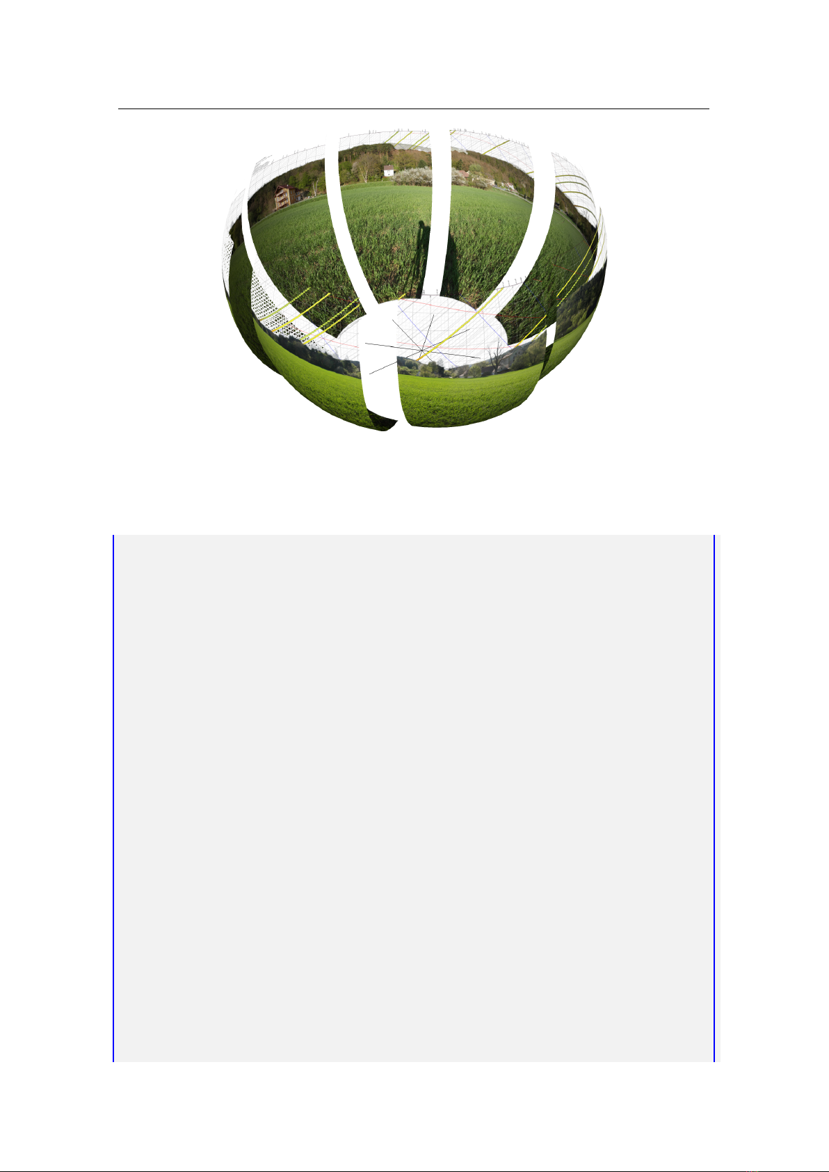
7.2 Creating Panorama Photographs for Stellarium 85
Figure 7.3: Zenit “Horizon 202” panorama camera with rotating lens for 35mm film. (Source:
Wikipedia, “Horizon202” by BillC - Own Work. Licensed under CC BY-SA 3.0 via Wikimedia Commons -
https:
//commons.wikimedia.org/wiki/File:Horizon202.jpg)
Figure 7.4: Automated panorama head. (Source: Wikipedia
https://commons.wikimedia.org/wiki/Fil
e:Rodeon_vr_head_01.jpg)

86 Chapter 7. Landscapes
As a general recommendation, the images of a panorama should be taken from left to right, else please
accordingly invert some of the instructions given below.
There are several panorama making programs. Often they are included in the software that comes with a
digital camera and allow the creation of simple panoramas. Other software titles are available for purchase.
However, there is one cost-free open-source program that does everything we need for our task, and much
more:
7.2.2 Hugin Panorama Software
Hugin
8
, named after one of the ravens that sits on Odin’s shoulder and tells him about the world, is a
user-friendly catch-all package with graphical user interface that allows creating panoramas with a single
application. Actually, Hugin is a GUI application which calls several specialized sub-programs with fitting
parameters. The instructions are based on Hugin V2014.0 and 2015.0.
Typically digital images come in JPG format with information about camera, lens, and settings stored in
invisible metadata in the EXIF format. When Hugin reads such images, it can automatically derive focal
length, field of view, and exposure differences (exposure time, aperture, color balance) to create panoramas
as easily as possible.
After starting Hugin for the first time, select
Interface Expert
to release several options not visible to
“beginners”. In the Preferences dialog (
Files Preferences
), edit number of CPU to match the number of
cores in your computer and allow parallel processing. E.g., if you have an Intel Core-i7, you usually can set
up to 8 cores (4 cores with hyperthreading; but maybe leave one core for your other tasks while you wait for
a processing job?). If your PC is equipped with a modern programmable graphics card, you can enable its
use in the
Programs
tab with activating “Use GPU for remapping”.
After that, we are ready for creating our panoramas.
7.2.3 Regular creation of panoramas
The graphical user interface (GUI) consists of a main menu, symbols, and 4 tabs. We start on the tab Photos.
•
Add images. . .
Opens a file browser. Select the images which you want to stitch. Usually, lens data
(focal length, horizontal field of view
9
, . . . ) are read from the EXIF data. If those are not available
(e.g. cheap cameras, images scanned from film), you can enter those data on loading or later. The
images are now listed in the file list, and you can edit image parameters by marking one or more, and
then choosing from the context menu which you get from pressing the right mouse button. In case
you have used different lenses (or inadvertently used different focal lengths of a zoom lens), you can
assign separate lenses to the images.
Caveat: If you have resized the images, or produced copied on your RAW converter with non-native
resolution, the horizontal Field of View (FoV) in Hugin may be misidentified. You must edit lens
parameters and fill in the field of view from a full-size image. Else the first round of optimisation will
run into unsolvable trouble.
•
Select one image as position anchor (usually the center image), and one as exposure anchor (this can
be the same image). For our purpose, the anchor image should face south.
•
Next, we must find common feature points. The next field below provides the required settings. It
is recommended to use the CPFind command. To avoid finding control points in (moving) clouds,
select setting
Hugin’s CPFind + Celeste
10
. Then press
Create control points
. This opens a dialog box
in which you can see output of the selected feature point extractor. It should finish with a box telling
you the number of identified points. In rare cases some images cannot be linked to others, you will
have to manually add or edit feature points in those cases.
•
Now it’s time to start optimisations. On the
Geometric Optimimisation
combo, start with the button
Positions, incremental from anchor
, and press
Calculate
. Moments later, a first rough match is
available for inspection.
•
First open the Preview window (press
Ctrl
+
P
or click the blue icon). Assumed your images cover
the full horizon, the window shows an equirectangular area (360 degrees along the horizon and 180
degrees from zenith to nadir). The anchor image should be close to the image center, and the other
images should be already well-aligned to both sides. You can set the exact center point by clicking it
in the image. If the horizon appears badly warped, use the right mouse key and click on the horizon
8
http://hugin.sourceforge.net/
9
contrary to Stellarium, field of view (FoV) in Hugin means the horizontal extent in degrees.
10
If you forget this, you can remove cloud points by calling Celeste in the control point editor later

7.2 Creating Panorama Photographs for Stellarium 87
roughly near −90 or +90 degrees (halfway to the left or right).
•
Open the OpenGL preview window (press
Ctrl
+
Shift
+
P
or click the blue icon with GL inside).
This panel provides several important views:
–
The
Preview
tab is similar to the non-OpenGL preview. You can display an overlay of the
control points, which are colored according to match quality. Also, with button
Identify
activated, you see the overlapping image frames when you move the mouse over the image.
– The
Layout
tab helps finding links between images.
– The
Move/Drag
dialog may help to interactively adjust a panorama.
Sometimes the preview image may however be distorted and unusable.
•
Open the Control Points Table dialog (press
F3
or click the “table” button). Here you see the points
listed which link two images. Clicking a column label sorts by this column. It is recommended that
only neighboring overlapping images should be included here. If you have very large overlap, it is
possible that points are found between two images which are not directly adjacent. In the OpenGL
preview window, you can use the
Preview
or the
Layout
tabs to identify those image pairs. Such
points should be deleted. In the point table, click on columns “Right Img.”, then “Left Img.”, and then
find pairs like 0/2, 1/3, 2/4 etc. Mark those lines, and delete the points.
•
To re-run the optimisation, press the double-arrow icon or the
calculate
button in the Optimise/Geo-
metric area.
7.2.3.1 Preliminary Geometric Optimisation
Now the (usually) longest part begins: Iterative optimisation of the photo matchpoints. If your images were
taken on a panorama tripod head, there should only be very few bad matchpoints, e.g. those found on persons
or clouds
11
which have moved between photos. For handheld photos, the following considerations should be
observed.
The most important line which we want to create in all perfection is the visible horizon, where sky and
earth meet. The foreground, usually grassy or rocky, is of lesser interest, and stitching errors in those areas
may not even be relevant.
Therefore, matchpoints with large errors in the foreground can be safely removed, while, if necessary,
points on the horizon should be added manually. Use the
Control Points
tab, select adjacent images (start
with 0 on the left and 1 on the right side), and delete the worst-fitting matchpoints closest to the camera (near
the bottom of the images). We now start a long phase of re-optimizing and deletion of ill-matching points as
long as those are far from the horizon. When all near matchpoints are deleted, the result should already look
not too bad.
For continued optimisation, the number of parameters to optimize can be extended. To begin, I
recommend
Positions and View (y, p, r, v)
, which may find a new focal length slightly different from the data
in the EXIF tags. Again, delete further foreground points. If after a few rounds you still have bad point
distances, try
Positions and Barrel Distortion (y, p, r, b)
to balance distortion by bad optics, or even go up to
Everything without translation
. Optimisation can only reach perfect results if you did not move between
exposures. Else, find a solution which shows the least error.
In case you took your photos not on a tripod and moved too much, you may even want to play with the
translation options, but errors will be increasingly hard to avoid.
Using Straight Edges as Guides
If the panorama contains straight lines like vertical edges of buildings, these can be used to automatically
get a correctly leveled horizon: Vertical lines are mapped to vertical lines in equirectangular panos! In the
Control Points
tab, select the image with the vertical edge in both subframes, and mark points on the vertical
edge. (switch off auto-estimate!). Likewise, horizontal lines may help, but make sure lines like rooves are
perpendicular to your line of view, else the perspective effect causes an inclination.
Multi-ring Panoramas
If you are trying to create a panorama with several rings (horizon, one or two rings below, and nadir area),
you must try to create/keep control points that best give a result without visible seams. In this case, and esp.
if you have only used a regular tripod or even dared to go for a free-handed panorama, you may observe that
it is best to remove control points in neighboring photos in the lower rings, but keep only the “vertical” links
between images with similar azimuth.
In total, and if the foreground is not important but only grassy or sandy, the rule of thumb is that the
horizon images must be strongly linked with good quality (small errors), while images in the lower rings
should be linked mostly to their respective upper photos, but not necessarily to the images to its sides. The
11
You should have created control points with the Celeste option!
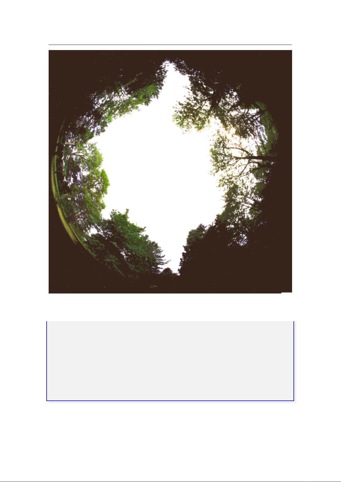
88 Chapter 7. Landscapes
resulting panorama will then show a good horizon line, while stitching artifacts in a grassy or otherwise only
decorative ground will usually be acceptable and can, if needed, be camouflaged in post-processing.
This optimization and editing of control points is likely a longish iterative process, and these are the late
night hours where you will finally wish you had used a panorama head. . .
7.2.3.2 Masking
If you have images with overlapping areas, you can usually not force Hugin to take pixels from the image
which you find best. you can however mask off an area from an image which you don’t want to see in the
output under any circumstances, e.g. a person’s arm or foot in one image. Just open the image in the
Mask
tab and either press
Add new mask
and draw the mask polygon covering the unwanted area, or use the crop
settings to define rectangular areas to use.
7.2.3.3 Exposure disbalance
In the
Photos
tab, select
Photometric parameters
on the right side. The EV column lists the Exposure Value.
If you see disbalance here and in the preview window, you can run a photometric optimization with the
lowest button on the
Photos
tab. Simply select Low dynamic range and press
Calculate
. The preview
should now show a seamless image. If all else fails, you can edit the EV values directly.
Advanced photographers may want to correct exposures in their RAW images before creating JPG or
TIF images to combine with Hugin. This unfortunately may create exposure disbalance because the EXIF
tags may not be adjusted accordingly, so based on different exposure/f-stop combinations Hugin may think
it has to re-balance the values. In these cases, don’t run the photometric optimizer. Some image exposure
values have to be changed manually, and the effect supervised in the preview window. Usually the smooth
blending in the subprogam enblend called by Hugin will hide remaining differences.
7.2.3.4 Stitching
When you are happy with the panorama in the preview window and the match-points promise a good fit, it is
time to finally create the panorama image. Hugin can create a large number of different projections which
all have their application. For Stellarium, we can only use the equirectangular projection. You still have 2
options:
spherical
landscapes (see 7.1.3) require single equirectangular images, the maximum size depends on your
graphics hardware and Qt limitations and is likely not larger than 8192× 4096 pixels.
old_style
landscapes (see 7.1.4) can use several textures for the ring along the horizon, and one image for
the nadir zone. If you need high resolution, you should aim for creating this one.
Sometimes, creating the nadir zone is difficult: this is where usually the view is blocked by the tripod,
and we are not interested in views of tripod or our own feet. For our purpose it is usually enough to fill in
the feet area using the clone stamp, or a monochrome color, or, for
old_style
landscapes, you can instead
insert an oriented site map or wind rose.
There is a button
create optimal size
in Hugin. It may recommend a panorama width around 13.000
pixels for an average camera and photos taken with a wide-angle lens. Increasing this size will most likely
not lead to higher optical resolution! The panorama width which you can most usefully create depends on
the resolution of the source images (which leads to the result given by Hugin) and on your needs. If you need
arc-minute resolution, you would aim for
360× 60 = 21600
pixels, which cannot be loaded into graphics
memory in a single piece, i.e., is too large for Stellarium, and must be configured as
old_style
landscape.
In this case, 10 or 11 tiles of 2048 × 2048 pixels (totalling 20480 or 22528 pixels) is the closest meaningful
setting, i.e., you could create an image of 20480 pixels width and cut this into usable pieces. Usually, a
size of
4096× 2048
or
8192× 4096
pixels (for better computers) is enough, and can be used in a
spherical
landscape.
We have to edit the file after stitching, therefore select creation of an image in the TIFF format. LZW
compression is non-lossy, so use this to keep file size reasonably small.
For regular images, it is enough to create “Exposure corrected, low dynamic range”. If you have a
problem with persons that have moved between your images, you may want to post-process the final result
with import of the distorted sub-images and manually defining the best blending line. For this, find the
“Remapped Images” group and again activate “Exposure corrected, low dynamic range”.
Now, press the
Stitch!
button in the lower right corner. This opens a helper program which supervises
the stitching process. Depending on your computer and size of the image, it will require a few minutes of
processing.
In case stitching fails with a cryptic error message, try to add the option --fine-mask to the enblend
options.
Store a copy of the Hugin project file to always be able to go back to the settings you used to create the

7.3 Panorama Postprocessing 89
last panorama. We will get back to it when we want to make a truly calibrated panorama (see 7.3.3).
7.3 Panorama Postprocessing
The image created has to be further processed to be used in Stellarium. The most obvious change is the
need for a transparent sky, which we can easily create in programs like Adobe Photoshop or the free and
open-source GIMP. I will describe only the free and open-source solution.
After that, we have to bring the image into shape for Stellarium, which may include some trimming.
While we could also slice an image with interactive tools, higher accuracy and repeatable results can be
achieved with command-line programs, which makes the ImageMagick suite the tool of our choice.
7.3.1 The GIMP
The GIMP (GNU Image Manipulation Program) has been developed as free alternative to the leading
commercial product, Adobe Photoshop. While it may look a bit different, basic concepts are similar. Not
everybody can (or wants to) afford Photoshop, therefore let’s use the GIMP.
Like Photoshop, the GIMP is a layer-aware image editor. To understand the concept, it is easiest to
imagine you operate on a growing stack of overhead slides. You can put a new transparent slide (“layer”) on
top of the stack and paint on this without modifying the lower layers.
A few important commands:
Zooming
Ctrl
+
Mouse Wheel
Layer visibility and transparency
Make sure to have layer dialog shown (
Windows Dockable Dialogs
).
A gray bar indicates opacity for the currently active layer. Note the mouse cursor in this opacity
bar (often also called transparency bar): near the top of the bar the upward pointer immediately sets
percentage. A bit lower the pointer looks different and can be used for fine-tuning.
The most obvious post-processing need for our panorama is making the sky transparent. The optimal
tool usually is the “Fuzzy Select”, which is equivalent to the “Magic Wand” tool in Photoshop. Simply
mark the sky, and then delete it. The checkerboard background indicates transparent pixels.
It sometimes helps to put an intensive bright red or blue background layer under the panorama photo to
see the last remaining clouds and other specks. In the layer dialog, create a new layer, bucket-fill with blue
or red, and drag it in the layer dialog below the pano layer. Write-protect this layer, work on the image layer,
and before exporting the image layer with transparent sky to PNG, don’t forget to switch off the background.
We need this layer functionality especially to align the panorama on a calibration grid, see section 7.3.3.
7.3.2 ImageMagick
ImageMagick (IM)
12
can be described as “Swiss Army Knife of image manipulation”. It can do most
operations usually applied to images in a GUI program, but is called from the command line. This allows
also to include IM in your own command scripts
13
. We will use it to do our final cut and resize operations. I
cannot give an exhaustive tutorial about more than a few of IM’s functions, but the commands given here
should be enough for our purpose.
To open a command window (console, a.k.a. DOS window), press the Windows key and enter
cmd
, then
press . (On Linux and Mac, you surely know how to open a console window.)
There are some things you might need to know:
•
The command line is not your enemy, but a way to call expert tools.
•
The Windows command line processor cmd.exe is far from user friendly.
•
There are remedies and alternatives. See notes on clink (7.5.3) for a considerable improvement, and
WSL (7.5.4) for experts.
7.3.2.1 Command-line magick for spherical landscapes
Let’s start with the commands for final dressing of an equirectangular panorama to be used as spherical
landscape which has been created in size
4096× 2048
, but where you have seen that nothing interesting is in
the image above 11.25°. This means we can cut away the sky area and compress the image to
4096× 1024
to
save graphics memory.
14
12
https://www.imagemagick.org/
13
These may typically be .BAT files on Windows, or various shell scripts on Linux or Mac.
14
Most modern graphics cards no longer require the “powers of two” image sizes, but we keep this practice to increase
compatibility.

90 Chapter 7. Landscapes
To understand the numbers in the example, consider that in a panorama image of
4096× 2048
pixels,
1024 pixels represent 90°,
512px = 45
°,
256px = 22.5
°,
128px = 11.25
°. To keep a top line of
11.25
°, we
keep an image height of 1024+ 128 = 1152px, but the crop starts at pixel Y = 1024− 128 = 896.
conver t lan dscape . png - crop 4096 x1152 +0+896
- resize 4096 x1024 ! la ndscape _crop ped . png
Note the exclamation mark in the -resize argument, which is required to stretch the image in a non-
proportional way.
Alternatively, you can operate with IM’s “gravity”, which indicates the corner or edge geometric offsets
are referred to. Given that we want the lower part of the image to exist completely, you only need to compute
the size of the cropped image:
conver t lan dscape . png - gra vity SouthWe st - crop 4096 x1152 +0+0
- resize 4096 x1024 ! la ndscape _crop ped . png
You still need the addition
+0+0
in the -crop option, else the image will be cut into several pieces. In the file
landscape.ini, you then have to set maptex_top=11.25.
7.3.2.2 Command-line magick for old_style landscapes
Let us assume we want to create a high-resolution landscape from a pano image of width 16384 which we
have carefully aligned and calibrated on an oversized grid template that also shows a measured horizon line
(see 7.3.3). Usually it is not necessary to create the full-size image, but only the horizon range, in this high
resolution. Assume this image has been aligned and justified on our grid image and is
HEIGHT
pixels high,
the left border is at pixel
X_LEFT
, and top border (i.e., the point where relevant content like the highest tree is
visible) is on pixel
Y_TOP
. Assume our graphics card is a bit oldish or you aim for maximum compatibility,
so we can load only textures of at most 2048 pixels in size. Given that the horizon area usually only covers a
few degrees, a vertical extent of
2048px
seem a pretty good range for that most interesting zone. The ground
can then be filled with some low-resolution image of grass, soil, or a properly oriented site map, or you can
use Hugin to create a ground image (and using the maximum of
2048× 2048
also here usually is far more
than enough).
In GIMP (or Photoshop, . . . ), we must find the values for
X_LEFT
,
Y_TOP
and
HEIGHT
.
HEIGHT
is being
resized to 2048, strictly, by the exclamation mark in the resize command. We can create our image tiles
now with this singular beast of a command line (write all in 1 line!), which puts our files directly into
STELLARIUM_LANDSCAPEPATH/LANDSCAPE_NAME:
conver t PANO . png - crop 16384 xHEIGH T + X_LEFT + Y_TOP + repage
- resize 16384 x2048 !
- type TrueC olorM atte -depth 8
- crop 2048 x2048 + repage
png : ST ELLARIU M_ LANDSCA PE PATH / L ANDSC APE_NAME / Horiz -% d. png
This creates 8 images. See section 7.1.4 for the
landscape.ini
where these images can be referenced.
Don’t forget to read off top and bottom lines (altitudes in degrees) from your grid, the vertical extent will
form the decor_alt_angle, and the bottom line the decor_angle_shift entries in this file.
Creating a ground image for old_style landscapes
When you want a good ground image for an
old_style
landscape from your panorama and not just fill the
groundtex
with a monochrome texture or a map, you have to create a ground view in Hugin. But you may
have already created a huge pano! This can also be used as source image, and a ground shot can be extracted
with a reversed operation. In principle, all you need to know is the field of view around the nadir. Figure 7.5
shows a simple configuration file.
Say, the side panels extend down to
decor_angle_shift=-44
degrees, which means you must close
the ground with a Nadir
FoV = 2× (90− 44)= 92
. For maximum compatibility, we will again make an image
of width and height both 2048
px
. These values can be found in the
p
line in Figure 7.5. The
i
line describes
the input image, which is our full equirectangular pano of width
w= 16384
and height
h= 8192
. The last
argument of that line is the image file name.
For processing, we do not use the Hugin GUI, but simply the command line. The actual program to call
is nona. If your stitched panorama is a 16-bit TIFF, nona will also make a 16-bit image, but our textures are
limited to 8-bit PNGs. We apply our most useful tool, convert from the ImageMagick suite.
nona -v -m PNG ground . pto -o ground . png
conver t ground . png - depth 8 gr oun d_8b it . png
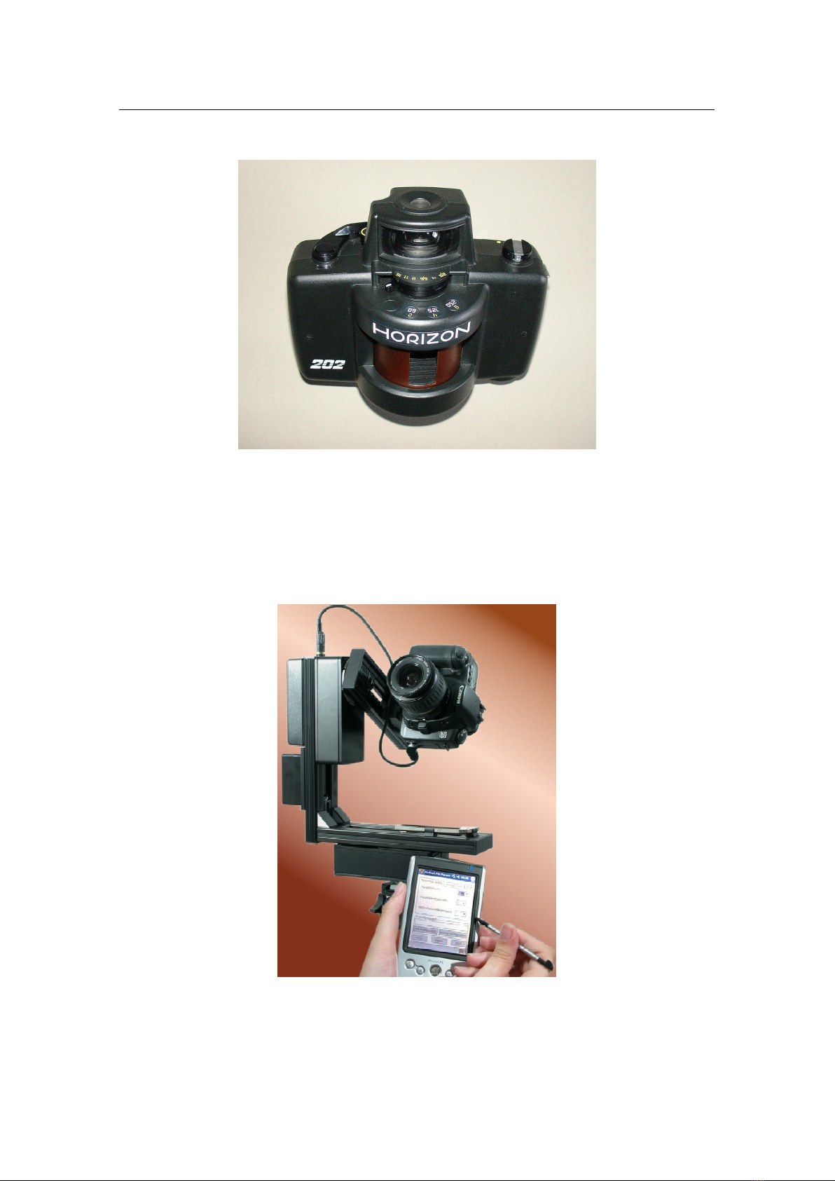
7.3 Panorama Postprocessing 91
# hugin project file
# h ugin_ ptove rsion 2
p f0 w2048 h2048 v92 E0 R0 n" TIFF_m c : LZW r : CROP "
m g1 i0 f0 m2 p0 .00 784 314
# image lines
# - hugin c ropF act or =1
i w16384 h8192 f4 v360 Ra0 Rb0 Rc0 Rd0 Re0 Eev0 Er1 Eb1 r0
p90 y0 TrX0 TrY0 TrZ0 Tpy0 Tpp0 j0 a0 b0 c0 d0 e0 g0 t0
Va1 Vb0 Vc0 Vd0 Vx0 Vy0 Vm5 n" Eqir ect_P ano36 0 . png "
Figure 7.5: Project file
ground.pto
usable to create the ground image with Hugin or, on the
command line, its nona stitcher. The last line, starting with
i
, has been wrapped, but must be 1 line.
The file ground_8bit.png is then used in the groundtex field on landscape.ini.
7.3.3 Final Calibration
The creation of a calibrated panorama (which can be regarded as dependable proxy for further measurements
taken inside Stellarium) requires reference measurements to match the photos against. We must take
azimuth/altitude measurements with a theodolite or total station, in the optimal case along the full horizon,
and in addition I recommend to take azimuth and altitudes of some distinct features along the horizon which
must also be visible in the photographs: mountain summits, electrical towers, church towers, . . .
I recommend you create grid templates of the sizes you are going to create, e.g. 4096, 8192, 16386 and
20480 pixels wide with some diagram tool. On these, you can then also draw the measured horizon line.
Now, load a panorama on top of this in the GIMP, i.e., copy it into a separate layer over the grid image,
and set it semi-transparent.
Try to align the center of the image (where the geometric anchor has been defined; remember: this
should be the image pointing south!) with the measured horizon line or the distinct features.
The optimal solution consists of a photo panorama which aligns perfectly with the measured line and
features. We now have to iteratively bring deviations to a minimum. The process depends on processor
speed, image size, your training and – most of all – your requirements in accuracy!
In the GIMP, load your grid image with horizon line. Now select
File Open as Layers. . .
, load your
photo panorama, and then set layer transparency in the
Layers
dialog to about 50%.
Select the double-arrow tool to move the panorama via mouse drag and cursor keys over the grid, and
align the outline of the photo horizon’s southern point with the measured line. Now it’s time to estimate the
quality of the panorama.
In Hugin’s
Photos
tab, select the
Positions
view on the right side. Now you see “Yaw”, “Pitch” and
“Roll” values of camera-to-world orientation listed in the photos list. It should now be possible, by changing
the values only for the anchor image and re-optimizing, to come to a panorama with only minimal error. In the
process, start with Optimizing
Positions incremental from anchor
, then go for view and barrel optimization,
and so on. Always try to remove foreground match points which have large error and are irrelevant for the
task to match the horizon. Those are especially cross-matches of horizon and sub-horizon rows of images.
Only vertically and horizontally adjacent images should be required to match. For handheld panoramas, also
links between adjacent images in the non-horizontal rows are usually too erroneous to be useful, just remove
these match points. Use the
Layout
tab in the Fast Panorama Preview to see the relations between images
(Fig. 7.6): Red lines have big errors, green lines are good, thin gray lines indicate possible overlap without
specified match points. After each optimization step, export a new pano image, load as layer in GIMP, and
check again.

92 Chapter 7. Landscapes
Figure 7.6: Hugin’s Fast Panorama Preview can be used to check which images are connected to its
neighbors. Most important are good matches along the horizon, the images in the lower rows are
clearly less important. If captured on a tripod, they should still match.
Basic rules to observe (use obvious inverses).
•
If image aligns well in azimuth but overshoots the grid to the right: Increase yaw accordingly
(0.022°/pixel if image is 16384 pixels wide).
•
If the north end (left and right borders) is higher than the southern contact point: Increase pitch
angle.
•
If north and south points are OK, but the western (right) half is higher than the eastern (left) half:
Increase Roll angle.
The corrections required for pitch and roll may be surprisingly small!
Within a few rounds of adjustments, panorama creation, adding as layer in the image editor, and
comparing to the reference data, you should achieve a match to fit your needs.
In case you have taken photographs in several rings but without a panorama tripod, you may have to first
align only the horizontal images (deselect the lower images to exclude from optimization), and when the
horizon ring is aligned perfectly, deactivate further optimization in Hugin for those photos while “attaching”
(optimizing) the lower photos. In Hugin’s
Photos
tab, select
Optimize Geometric Custom Parameters
.
This opens an extra tab
Optimizer
, where you can fine-tune your needs: Switch off all variables for the
photos in the horizon ring, and make sure the lower photos fit in the preview after optimization.
It may even help to define that the lower rows have been taken with a different Lens, so the field of view
and distortion settings of the horizon row will be used as it had been found during the horizon-only match.
By now you should have enough experience what level of error may be acceptable for you.
7.3.4 Artificial Panoramas
You do not have to visit a site to create a panorama from your own photographs. There is dedicated software
that can process free and proprietary geodata.
A classic for archaeoastronomers is Andrew Smith’s Horizon
15
which can process SRTM 1” data which
are freely available.
A web service similar to HeyWhatsThat (see 7.1.2.1), PeakFinder
16
, creates a polygonal line and
black/white landscape feature renderings and also allows downloading the horizon as installable landscape
15
urlhttp://www.agksmith.net/horizon/
16
https://www.peakfinder.com
7.3 Panorama Postprocessing 93
for Stellarium. A great feature of this service is the excellent gazetteer (peak identification) also visible on
the website.
BRIAN DOYLE has created another online service, Skyliner
17
, computing a panorama in the web browser.
A gazetteer can be created manually. A similar website that can also export Stellarium landscapes is DAVID
HOYLE’s Panorama
18
. He also released his program, which can process SRTM and even Lidar data on
Github
19
.
I have created a website
20
where you can enter geographical coordinates and download a file
pano.kml
which helps with image creation from Google Earth imagery. Store this file for a site, let us call it MYPLACE,
into a new directory GE_MYPLACE inside your landscapes directory.
Store all scenes visible from the respective viewpoint MYPLACE as picture into one common folder
in your
landscapes/GE_MYPLACE
under the viewpoint name, e.g.,
75-30.jpg
, which means 75 degrees
from Nadir, azimuth 30 degrees. Also, double-click the pano entry or the marker in Google Earth to
open a window with the basic content of your
landscape.ini
. Copy and paste from there into a new
file
landscape.ini
and adjust the obvious entries. Complete as required with the entries described in
section 7.1.3.
On loading of the images, Hugin will not be able to detect any EXIF lens data and ask you for the
horizontal field of view. Enter 60 degrees, which is the standard value for Google Earth screenshots
21
.
The viewpoint names translate almost directly to the yaw and pitch angles which you can enter in the
image list in Hugin’s
Photos
tab. For example, switch to the
Positions
display on the right window edge in
the
Photo
tab, mark all images that start with
25-
and assign a pitch angle of
−90+ 25 = −65
. The second
part of the names is directly the azimuth. In this case, don’t run the optimizer, but you can immediately
set an output resolution and stitch (see 7.2.3.4). To get rid of the image decorations (compass etc), apply
masks
22
. Post-processing steps are the same as for photo-panoramas: make sky invisible, crop, etc.
It is also interesting to switch on the 3D buildings layer before creating the images. If temples or other
buildings are accurate, this will give an even closer approximation to what would be visible on-site. Note
however that not every building will be modelled in usable quality, and that usually vegetation is not included
in the 3D buildings layer. Also, if you are too close to buildings, they may be cut away by the near clipping
plane of the rendering.
These images, based on Google Earth imagery and the SRTM topographic model, seem usable as first
rough approximation to a photo-based or surveyed panorama. Note that it is definitely not accurate enough
for representing nearby horizon features or critically important mountain peaks, and please note that Google
has image copyright which at least requires you to acknowledge when displaying these pictures.
7.3.5 Nightscape Layer
Since version 0.13, Stellarium can simulate artificial illumination, like streetlamps, bright windows, or the
skyglow over cities (Zotti and Wuchterl, 2016). One way to create this layer is to make 2 panorama series
during the day and night and process these in the same Hugin project to align those photos, and then stitch
two separate images by selecting either the daylight or the nighttime shots. The night panorama has to be
processed to remove stars, airplanes, etc.
The other way is a simple layer overpainted in the image processing program. As rough recommendation,
use several layers to prepare this feature:
•
Put a semitransparent black layer over your daylight image, this helps you to place your painted
pixels.
•
Paint windows, street lamps, signs, . . . . You may apply a layer style to produce some glow.
•
To draw an impression of more light in the atmosphere (city skyglow), use a gradient with some
brownish color. Generally the color depends on the appropriate mix of city lights (sodium, mercury
vapour, etc.). Note that on the city outskirts a simple vertical gradient will not work, towards the city
the horizon is much brighter. Use a huge but weak brush to make a more spotty sky.
•
Use the existing landscape as template for the layer mask for this gradient sky layer. (You want to
hide skyglow by leaves in the foreground!)
17
https://archaeoastronomyireland.github.io/skyliner/
18
https://www.standingstones.org/viewer.html
19
https://github.com/davidjhoyle/OpenPanorama
20
https://gzotti.github.io/panoCam.html
21
Note that if you work with Google Earth Pro, you can create different FoV!
22
There is a wide overlap in the images to allow generous trimming.

94 Chapter 7. Landscapes
•
If you want to add only a few lights to an
old_style
landscape, you need to provide only the panels
showing those lights. Just load a side panel for reference, place a new layer on top, and paint the
lights on windows, lamps etc. There is no light option for the ground texture. This makes
old_style
landscapes best suited for localized light pollution, not city skyglow.
The resulting image is then declared in the
maptex_illum
line of
landscape.ini
. Try also to balance
the global strength of light pollution with the
light_pollution
key, and a probable minimal brightness
with the minimal_brightness key.
Try to match the visual appearance, not necessarily what photographs may have recorded. E.g., the
Grossmugl sky shows horizon glow mostly towards the city of Vienna, where long-time exposures may
already be saturated.
The possibilities seem limited only by your time and skills!
7.4 Troubleshooting
If something does not work as described and Stellarium does not show your landscape as expected but maybe
just a bright magenta-colored box, don’t panic. Double and triple-check the entries in
landscape.ini
.
Make sure the texture is in PNG format and the file name is correct. Check the logfile for error messages.
If the image is too large, it will be re-scaled on loading, but it is more efficient to keep images as small as
required. Only few systems can use textures larger than
16384× 16384
Pixels. If you need high resolution,
use the old_style type (see section 7.1.4).
7.5 Other recommended software
Here is a short collection of other useful programs for (panorama) image manipulation and other tasks on
Windows.
7.5.1 IrfanView
IrfanView is a free image viewer for Windows with many options. It can show almost any image format,
including several camera RAW formats, in windowed and full-screen mode. It is definitely preferable over
any image viewer built into Windows. Unfortunately however, it has no panorama viewer function!
7.5.2 FSPViewer
FSPViewer
23
by Fulvio Senore is an excellent panorama viewer for equirectanglar images. Images centered
along the horizon can be viewed directly, while settings for images with different minimum and maximum
angles, as well as “hotspots” (similar to hyperlinks) which move to neighboring panoramas, can be configured
in an .FSV text file like figure 7.7.
ImageNa me = H orizo n_Ros enbur g . jpg
Windo wTi tle = Hori zon_R osenb urg
hFov =70
# Formula : HP =100*( h/2 - upper )/( lower - upper ) in Hugin crop , or
# HP =100* zer oRow / img Height
Ho rizon Position =33.8
Figure 7.7: FSP configuration file (example)
7.5.3 Clink and GNUWin32
Clink
24
is a command line enhancement for Windows developed by Martin Ridgers. If you have ever worked
under a Linux bash-like command line, you will easily feel that Windows’ cmd.exe is extremely limited.
Clink provides several useful features, most notably a really usable command-line completion. It is not
essential for our tasks, but a general improvement of usability of the Windows command line which else has
not caused me any trouble.
23
Further details are available on its home page http://www.fsoft.it/FSPViewer/.
24
http://mridgers.github.io/clink/

7.5 Other recommended software 95
Compared to Linux, the command line of Windows can still be a humbling experience. None of the
wonderful helpers taken for granted on Linux are available. Many of the nice tools known and taken for
granted by Linux users (make, sed, awk etc.) have also been made available as standalone commands for
Windows. If you don’t need the inline scripting capabilities in
Makefile
s which you would get from a more
complete Linux installation but just want to call awk or sed inside your .BAT scripts, maybe this is enough.
7.5.4 WSL – Windows Subsystem for Linux
Finally, the 64-bit editions of Windows 10 come with an optional feature that allows you to install a complete
Linux distribution like Ubuntu inside your Windows system. Combined with an X11 server like XMing
25
,
you can even run graphic applications like Stellarium, and all the command-line tools are available.
25
https://sourceforge.net/projects/xming/


8. Deep-Sky Objects
Since version 0.10.0 Stellarium uses the “json” cataloguing system of configuring textures. At the same time
the Simbad online catalogue was added to the search feature, making the catalog somewhat redundant and
used now only as a first search point or if there is no Internet connection.
If the object has a name (not just a catalogue number), you should add one or more records to the file
.../nebulae/default/names.dat
(where
...
is either the installation directory or (preferably) the user
directory). See section 8.1.2 Modifying names.dat for details of the file format.
If you wish to associate a texture (image) with the object, you must add a record to the file
.../nebulae/default/textures.json
See section 8.1.3 for details.
If you wish to associate an outline with the object, you must add the series of lines to the file
.../nebulae/default/outlines.dat. See section 8.1.4 for details.
8.1 Stellarium DSO Catalog
Stellarium’s DSO Catalog contains over 94000 objects
1
(up to
15.5
m
for galaxies) and is available for end
users as collection of files:
catalog.txt Stellarium DSO Catalog in ASCII format for editing data
catalog.dat Stellarium DSO Catalog in zipped binary format for usage within Stellarium
2
names.dat List of proper names of the objects from file catalog.dat
An edited ASCII file can be converted into binary format through enabling an option in the file
config.ini (See 5.4):
[ devel ]
co nvert_d so_ca talog = true
The file
catalog.txt
should be put into the directory
.../nebulae/default/
and you should create
an empty file
catalog.pack
to storing the binary catalog. After converting the data into binary format you
should gzip them by the command
gzip -nc catalog . pack > catalog . dat
Stellarium DSO Catalog contains data and supports the designations for follow catalogs
3
:
NGC New General Catalogue
IC Index Catalogue
M Messier Catalog
1
An extended edition of this catalog with over one million objects may be downloaded and installed manually (see
section 5.5.2).
2
The file name
catalog-VERSION.dat
is used for extended edition of DSO Catalog, where VERSION is version
of catalog.
3
Abell Catalog of Planetary Nebulae was added in v0.18.2 and removed in v0.20.1

98 Chapter 8. Deep-Sky Objects
C Caldwell Catalogue
B Barnard Catalogue (Barnard, 1927)
SH2 Sharpless Catalogue (Sharpless, 1959)
vdB van den Bergh Catalogue of reflection nebulae (van den Bergh, 1966)
RCW
A catalogue of H
α
-emission regions in the southern Milky Way (Rodgers, Campbell, and
Whiteoak, 1960)
LDN Lynds’ Catalogue of Dark Nebulae (Lynds, 1962)
LBN Lynds’ Catalogue of Bright Nebulae (Lynds, 1965)
Cr Collinder Catalogue (Collinder, 1931)
Mel Melotte Catalogue of Deep Sky Objects (Melotte, 1915)
PGC HYPERLEDA. I. Catalog of galaxies
4
UGC The Uppsala General Catalogue of Galaxies
Ced Cederblad Catalog of bright diffuse Galactic nebulae (Cederblad, 1946)
Arp Atlas of peculiar galaxies
5
(Arp, 1966)
VV
The catalogue of interacting galaxies by Vorontsov-Velyaminov (Vorontsov-Velyaminov,
Noskova, and Arkhipova, 2001)
PK Version 2000 of the Catalogue of Galactic Planetary Nebulae (Kohoutek, 2001)
PN G The Strasbourg-ESO Catalogue of Galactic Planetary Nebulae
6
(Acker et al., 1992)
SNR G A catalogue of Galactic supernova remnants (Green, 2025)
Abell A Catalog of Rich Clusters of Galaxies (Abell, Corwin, and Olowin, 1989)
HCG Atlas of compact groups of galaxies (Hickson, 1993)
ESO ESO/Uppsala Survey of the ESO(B) Atlas (Lauberts, 1982)
vdBH Catalogue of southern stars embedded in nebulosity
7
(van den Bergh and Herbst, 1975)
DWB
Catalogue and distances of optically visible H II regions (Dickel, Wendker, and Bieritz,
1969)
Tr Trumpler Catalog
8
St Stock Catalog
Ru Ruprecht Catalog
vdB-Ha van den Bergh-Hagen Catalog (van den Bergh and Hagen, 1975)
Other
deep-sky objects without designations and sky regions — by formal rules objects from this
list are not included in any catalog known to Stellarium
Cross-index data for Stellarium’s DSO Catalog is partially obtained from “Merged catalogue of reflection
nebulae” (Magakian, 2003) and astronomical databases SIMBAD
9
(Wenger et al., 2000) and NED
10
.
Distances for some deep-sky objects obtained from “The Magellanic Cloud Calibration of the Galactic
Planetary Nebula Distance Scale” (Stanghellini, Shaw, and Villaver, 2008), “A 1.4 GHz Arecibo Survey
for Pulsars in Globular Clusters” (Hessels et al., 2007), “Distance measurements of LYNDS galactic dark
nebulae.” (J. Hilton and Lahulla, 1995) and “A Catalog of Parameters for Globular Clusters in the Milky
Way” (Harris, 1996).
Morphological class for many open clusters obtained from “Classification of open star clusters” (Ruprecht,
1966).
Visual magnitudes for Messier objects obtained from “Revised New General Catalogue and Index Catalogue”
by Dr. Wolfgang Steinicke (Version: 2 February 2021 — NI2021)
11
.
4
The PGC and UGC catalogs are partially supported
5
Arp, VV and PK was added in version 0.16.0
6
PN G, SNR G and Abell was added in version 0.16.1
7
vdBH and DWB was added in version 0.19.2
8
Tr, St, Ru and vdB-Ha was added in version 0.20.2
9
SIMBAD Astronomical Database — https://simbad.u-strasbg.fr/simbad/
10
NASA/IPAC Extragalactic Database (NED) — https://ned.ipac.caltech.edu/
11
Discovery and Cataloguing of Nebulae and Star Clusters —
http://www.klima-luft.de/steinicke/index
_e.htm
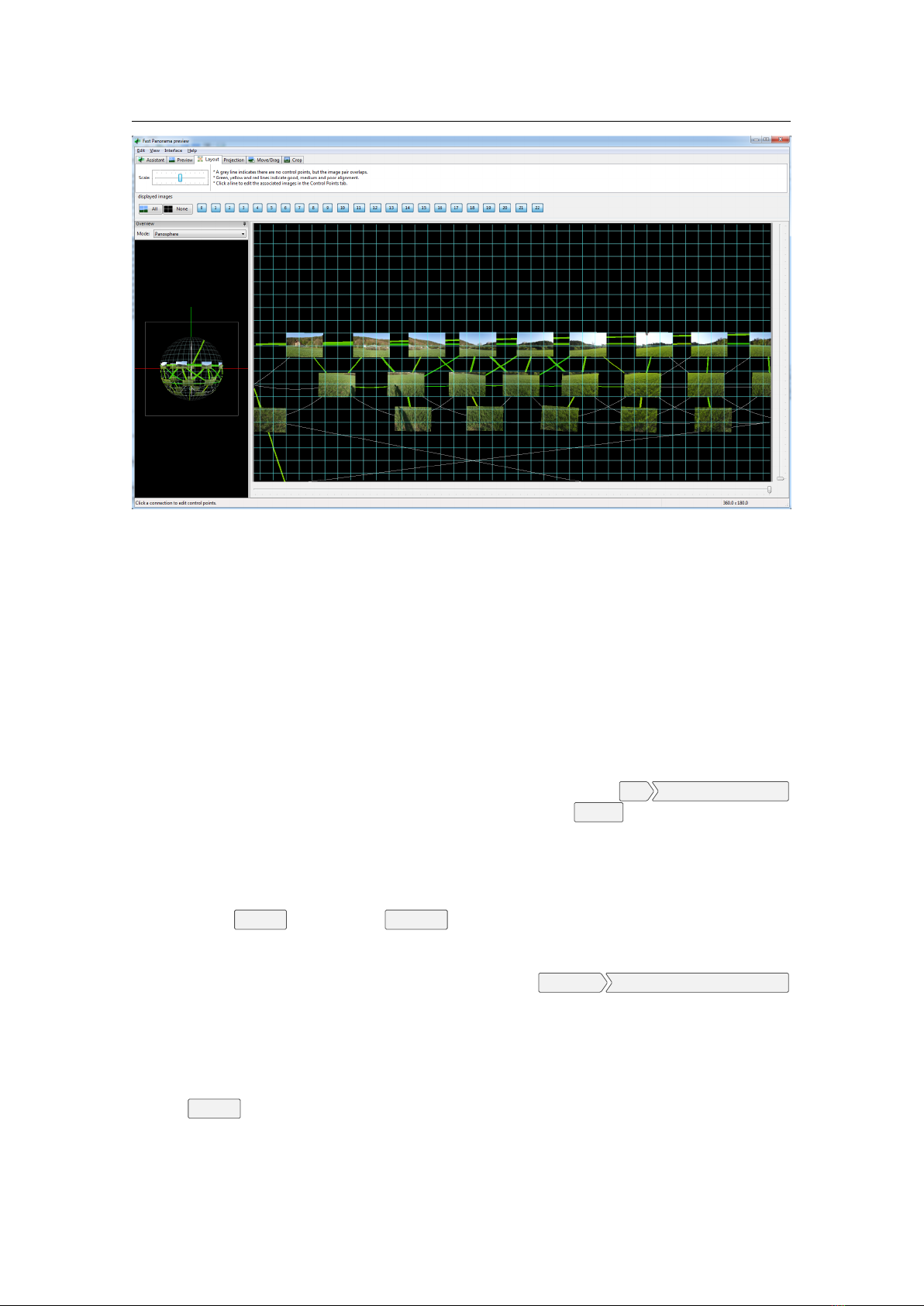
8.1 Stellarium DSO Catalog 99
8.1.1 Modifying catalog.dat
This section describes the inner structure of the files
catalog.dat
(binary format) and
catalog.txt
(ASCII format). Stellarium can convert ASCII file into the binary format file for faster usage within the
program.
Each line contains one record, each record consisting of the following fields with tab char as delimiter:
Column Type Description
1 integer Deep-Sky Object Identificator
2
float RA (decimal degrees)
3
float Dec (decimal degrees)
4
float B magnitude
5
float V magnitude
6
string Object type (See section 8.1.1.1 for details).
7
string Morphological type of object
8
float Major axis size or radius (arcmin)
9
float Minor axis size (arcmin)
10
integer Orientation angle (degrees)
11
float Redshift
12
float Error of redshift
13
float Parallax (mas)
14
float Error of parallax (mas)
15
float Non-redshift distance (Mpc for galaxies, kpc for other objects)
16
float Error of non-redsift distance (Mpc for galaxies, kpc for other objects)
17
integer NGC number (New General Catalogue)
18
integer IC number (Index Catalogue)
19
integer M number (Messier Catalog)
20
integer C number (Caldwell Catalogue)
21
integer B number (Barnard Catalogue)
22
integer SH2 number (Sharpless Catalogue)
23
integer vdB number (van den Bergh Catalogue of reflection nebulae)
24
integer
RCW number (A catalogue of H
α
-emission regions in the southern Milky Way)
25 integer LDN number (Lynds’ Catalogue of Dark Nebulae)
26
integer LBN number (Lynds’ Catalogue of Bright Nebulae)
27
integer Cr number (Collinder Catalogue)
28
integer Mel number (Melotte Catalogue of Deep Sky Objects)
29
integer PGC number (HYPERLEDA. I. Catalog of galaxies); partial
30
integer UGC number (The Uppsala General Catalogue of Galaxies); partial
31
string Ced identificator (Cederblad Catalog of bright diffuse Galactic nebulae)
32
integer Arp number (Atlas of Peculiar Galaxies)
33
integer VV number (The catalogue of interacting galaxies)
34
string PK identificator (Catalogue of Galactic Planetary Nebulae)
35
string
PN G identificator (The Strasbourg-ESO Catalogue of Galactic Planetary Nebu-
lae)
36
string SNR G identificator (A catalogue of Galactic supernova remnants)
37
string Abell identificator (A Catalog of Rich Clusters of Galaxies)
38
string HCG identificator (Atlas of compact groups of galaxies)
39
string ESO identificator (ESO/Uppsala Survey of the ESO(B) Atlas)
40
string vdBH identificator (Catalogue of southern stars embedded in nebulosity)
41
integer DWB identificator (Catalogue and distances of optically visible H II regions)
42
integer Tr identificator (Trumpler Catalogue)
43
integer St identificator (Stock Catalogue)
44 integer Ru identificator (Ruprecht Catalogue)
45
integer
vdB-Ha identificator (Uniform survey of clusters in the Southern Milky Way —
van den Bergh-Hagen Catalogue)
100 Chapter 8. Deep-Sky Objects
8.1.1.1 Types of Objects
Possible values for type of objects in the file catalog.dat.
Type Description
G Galaxy
GX
Galaxy
AGX
Active Galaxy
RG
Radio Galaxy
IG
Interacting Galaxy
GC
Globular Cluster
OC
Open Cluster
NB
Nebula
PN
Planetary Nebula
DN
Dark Nebula
RN
Reflection Nebula
C+N
Cluster associated with nebulosity
HII
HII Region
SNR
Supernova Remnant
SNC
Supernova Candidate
SNRC
Supernova Remnant Candidate
BN
Bipolar Nebula
EN
Emission Nebula
SA
Stellar Association
SC
Star Cloud
CL
Cluster
IR
Infra-Red Object
QSO
Quasar
Q?
Possible Quasar
ISM
Interstellar Matter
EMO
Emission Object
LIN
LINEAR-type Active Galaxies
BLL
BL Lac Object
BLA
Blazar
MOC
Molecular Cloud
YSO
Young Stellar Object
PN?
Possible Planetary Nebula
PPN
Protoplanetary Nebula
∗
Star
∗∗
Double Star
MUL
Multiple Star
SY∗
Symbiotic Star
EM∗
Emission-line Star
CLG
Cluster of galaxies
empty
Unknown type, catalog errors, Unidentified Southern Objects etc.
8.1.2 Modifying names.dat
Each line in the file
names.dat
contains one record. A record relates an extended object catalog number
(from catalog.dat) with a name. A single catalogue number may have more than one record in this file.
The record structure is as follows:
Offset Length Type Description
0 5 %5s Designator for catalog (prefix)
5
15 %d Identificator for object in the catalog
20 end %s Proper name of the object (translatable) [# references]
If an object has more than one record in the file
names.dat
, the last record in the file will be used for the
nebula label.

8.1 Stellarium DSO Catalog 101
8.1.2.1 Too many names?
Over the years, a large collection of names from many references has been added. DSO names are not
v 25.1
standardized and are generally not used by professional astronomers, but are often used for popularisation
of objects. Some of the collected names may be too fanciful for your taste. If you can identify that those
names that annoy you all come from a single or just a few entries of the reference list, you can exclude those
sources, and thus the names they bring. Note that if a fancy name comes from more than one book, you
would have to exclude all books to ban that name from your display.
To exclude entries, add the following key to config.ini:
[ astro ]
ne bu la_excl ud e_refer en ces = defaul t : ADI , DSC - HT
Here,
default
names the nebula set, and the comma-separated entries are references you want excluded
from nebulae/default/names.dat.
8.1.3 Modifying textures.json
This file is used to describe each nebula image. The file structure follows the JSON format, a detailed
description of which may be found at
www.json.org
. The
textures.json
file which ships with Stellarium
has the following structure:
serverCredits (optional) a structure containing the following key/value pairs:
short a short identifier of a server where the json file is found, e.g. “ESO”
full a longer description of a server, e.g. “ESO Online Digitized Sky Survey Server”
infoURL a URL pointing at a page with information about the server
imageCredits
a structure containing the same parts as a serverCredits structure but referring to the image
data itself
shortName an identifier for the set of images, to be used inside Stellarium
minResolution
minimum resolution, applies to all images in the set, unless otherwise specified at the image
level
maxBrightness
the maximum brightness of an image, applies to all images in the set, unless otherwise
specified at the image level
subTiles
a list of structures describing individual image tiles, or referring to another json file. Each subTile
may contain:
minResolution
maxBrightness
worldCoords
subTiles
imageCredits
imageUrl
textureCoords
shortName (name for the whole set of images, e.g. “Nebulae”)
miniResolution (applies to all images in set)
alphaBlend (applies to all images in set)
subTiles list of images. Each image record has the following properties:
imageCredits (itself a list of key/pairs)
imageUrl (e.g. file name)
worldCoords (a list of four pairs of coordinates representing the corners of the image)
textureCoords (a list of four pairs of corner descriptions. i.e. which is top left of image etc)
minResolution (over-rides file-level setting)
maxBrightness
Items enclosed in Quotation marks are strings for use in the program. Syntax is extremely important.
Look at the file with a text editor to see the format. Items in <> are user provided strings and values to suit
the texture and source.
{
" im a g e C r e d i t s " : { " short " : " <auth or name > " ,
" infoUr l " : " http :// < mysite . org > "
},
" imageUrl " : " <my P hoto .png > ",
" wo r l d C o o rds " : [[[ X0 , Y0 ] , [ X1 , Y1 ], [ X2 , Y2 ] , [ X3 , Y3 ] ]] ,

102 Chapter 8. Deep-Sky Objects
" te x t u r e C o o r d s " : [[[ 0 ,0] ,[1 ,0] ,[1 ,1] ,[0 ,1]]] ,
" mi n R e s o l u t i o n " : 0.2148 81046 3 ,
" ma x B r i g h t n e s s " : <mag >
},
where
worldCoords
Decimal numerical values of the J2000 coordinates (RA and dec both in degrees) of the
corners of the texture. These values are usually given to 4 decimal places.
textureCoords
Where 0,0 is South Left, 1,0 the South Right, 1,1 North Right, 0,1 North Left corners of the
texture.
minResolution UNDOCUMENTED VALUE! Sorry!
maxBrightness total object brightness, magnitude
Calculating of the coordinates of the corners of the images (plate solving) is a time consuming project
and needs to be fine tuned from the screen display. As most images will be two dimensional, display on
a spherical display will limit the size to about 1 degree before distortion becomes evident. Larger images
should be sectioned into a mosaic of smaller textures for a more accurate display.
8.1.4 Modifying outlines.dat
Each line in the file
outlines.dat
contains three “columns” of data for outline elements. The structure for
each line is as follows:
Offset Length Type Description
0 8 %d Right ascension (decimal hours)
10
18 %d Declination (decimal degrees)
20
60 %s Command
Coordinates for each point of outline is represented in the equatorial coordinate system for epoch J2000.0.
The possible values of the third “column” (Command) are:
start
This command marks a start point of the outline. This command should also contain the designation
of the deep-sky object.
vertex This command marks an intermediate point of the outline.
end This command marks an end point of the outline.
Example for outline of M42:
05.5 6401 -05.49880 start M 42
05.5 6759 -05.39201 vertex
05.5 6635 -05.31749 vertex
05.5 7158 -05.21922 vertex
05.5 7601 -05.21716 vertex
05.5 8830 -05.30164 vertex
05.5 9140 -05.34341 vertex
05.5 9028 -05.37076 vertex
05.5 9008 -05.38175 vertex
05.5 9581 -05.37159 vertex
05.5 9943 -05.47123 vertex
05.5 9912 -05.65838 vertex
05.5 9520 -05.73212 vertex
05.5 8490 -05.68102 vertex
05.5 6948 -05.57675 end
The format of the file
outlines.dat
is compatible with the similar file of the SkyChart (Cartes du
Ciel) planetarium.
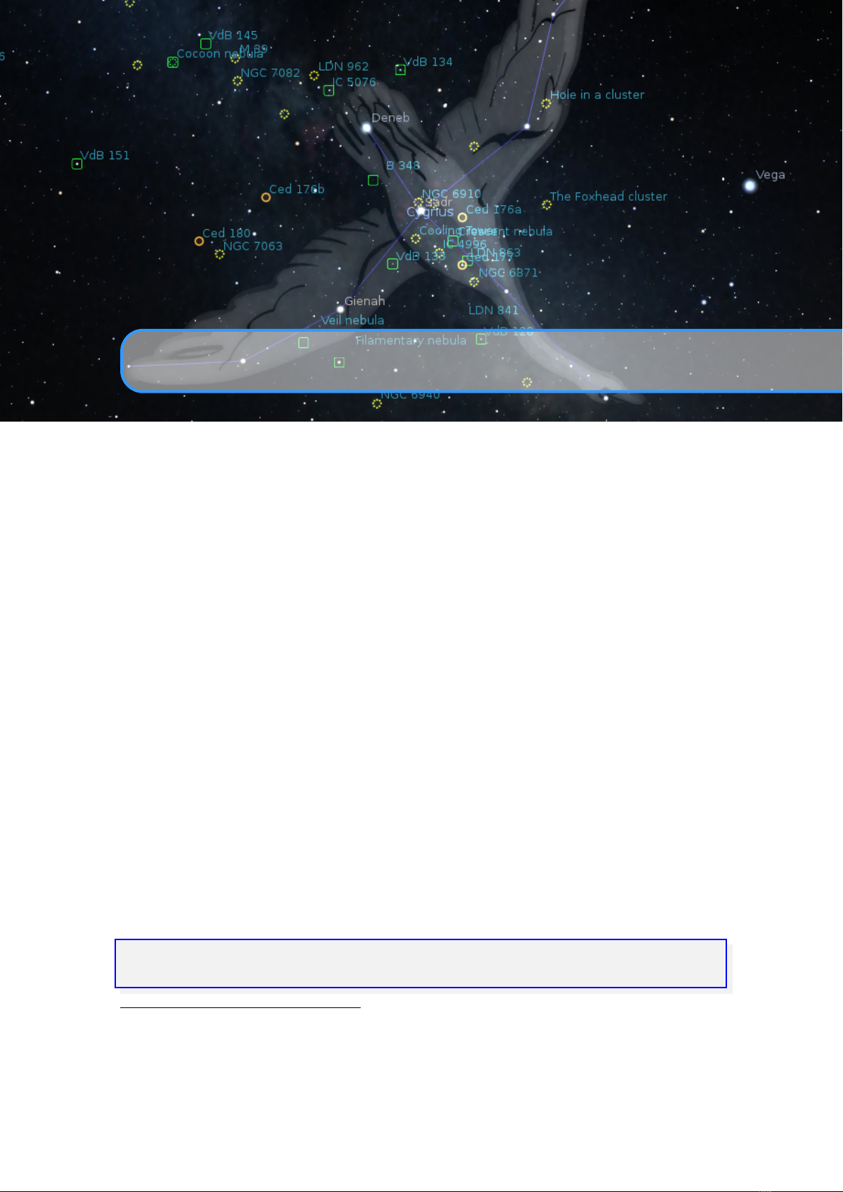
8.2 Adding Extra Nebula Images 103
8.2 Adding Extra Nebula Images
GLENN NEWELL
Figure 8.1: Screen shot of nebula images displayed in Stellarium
In previous versions of this guide, the technique for preparing Deep Space Object (DSO) images for inclusion
in Stellarium involved plate solving the image to find its center on the sky, and then calculating the corners
of the image in the World Coordinate System (WCS
12
) using the scale of the image, arc-seconds/pixel.
The problem with that approach is that it did not account for any spatial distortion in the image, due
to telescope optics or sensor tilt, etc. This resulted in a labor intensive manual process of trial and error to
adjust the WCS corners of the image until the stars in the image aligned with those displayed in Stellarium.
Fortunately, this problem has been solved for us by astronomers with similar needs, extending FITS
13
file headers to include information on how to map every pixel in an image correctly onto WCS coordinates.
This information can be added to your image when you plate solve it on nova.astrometry.net, or similar
services (local copies of astrometry.net, such as ansvr, or in Pixinsight, etc.). This system of correcting for
distortions in astronomical images was refined for the Spitzer Space Telescope
14
.
It is now possible to utilize this pixel to WCS transformation data included in plate solved images
to prepare images for Stellarium that map perfectly to the Stellarium sky without manual WCS corner
adjustments.
There are Python libraries, namely astropy and a related “channel” astroquery, that can automate some
or all of the needed steps, and there are both manual and fully automated scripts for that purpose available
on Stellarium’s GitHub site. These scripts can be run on Windows, Mac, or Linux platforms, using the
Anaconda Python distribution.
Nowadays, you can quickly plate solve deep space images and add them to the custom texture module
using the Nebula Textures plugin (see section 13.12).
8.2.1 Image requirements for inclusion in Stellarium
The final image must be aligned with the equatorial (J2000.0) coordinate system so that north is directly up
and not inverted side to side or up and down as can happen with photos taken with a diagonal mirror in the
path (In the WCS system, “Parity” must be 1.)
Next you will need to crop and/or re-scale the picture, setting the main feature at the center and making
the cropped size a power of 2, e.g. 64, 128, 256, 512, 1024 or 2048 pixels square (or elongated like
512× 1024
). If this requirement is not met, your textures may not be visible, or graphics performance may be
seriously impacted on some systems. Textures larger than 2048 may only be supported on high-end hardware.
Images must be in PNG format. When cropping, make sure you leave at least six prominent background
stars for plate solving). The next step is to process your photo to make the background black, really black.
12
https://fits.gsfc.nasa.gov/fits_wcs.html
13
The Flexible Image Transport System is the dominating image format used in astronomy.
14
https://www.cs.helsinki.fi/group/goa/viewing/viewtransf/viewTrans.html

104 Chapter 8. Deep-Sky Objects
This will ensure that your background will meld with the Stellarium background and not be noticed as ugly
gray square. Do not use “transparent” pixels available in the PNG format as they will show as white, not
black, in Stellarium.
Images covering more than 10 degrees of sky should be divided into separate images, and images with
pixel scales less than 1 arc-sec per pixel should be re-scaled so as to have a pixel scale of 1 arc-sec per pixel
or larger.
8.2.2 Processing requirements
•
Python 3.7 (Anaconda 64 bit installer
15
) During installation, follow directions, taking defaults to
install for just your user (vs. everyone on your computer)
•
Astropy (included in Anaconda)
•
Astroquery (latest version) To install on Windows, open an “Anaconda Prompt”. On Mac and Linux,
just open a terminal. At the prompt, enter:
pip install --pre --upgrade astroquery
•
For the fully automated process:
– An API Key from your account at https://nova.astrometry.net:
○ Create an account (or log in with google, etc.) at https://nova.astrometry.net
○ On the API tab, copy your API key (shown in green)
○
Using a text editor (e.g., Notepad++ on Windows, BBEdit on macOS), paste that key over
the
X
’s in
Stellarium_Nebulae_Images_Prep.py
’s
ast.api_key = ’XXXXXXXXXXXXXXXX’
•
For the more manual process:
–
Images plate solved at
https://nova. astrometry.net
(or Pixinsight – not yet tested) so
that WCS data is created
–
Graphics software to flip, rotate, scale, etc. and save as
.png
, e.g., Photoshop, GIMP, Pixinsight,
etc.
8.2.2.1 Script and Shortcut placement
Download the Python scripts from Stellarium’s site at Github
16
:
•
WCS_corners.py script
•
Stellarium_Nebulae_Image_Prep.py script
Windows
•
Place the two .py and .bat scripts into %USERPROFILE%\Anaconda3\
•
Place the two Shortcuts on your desktop or an astro tools folder (optional)
•
You can now drag and drop one or more images or
wcs.fits
files onto the shortcuts (or
.bat
scripts) for processing
Mac
•
Place the two
.py
script files in the
anaconda3
directory, which should be inside your home
directory (the directory with your username).
•
Place the two .app files on your desktop or an astro tools folder (optional)
•
You can now drag and drop one or more images or
wcs.fits
files onto the Automator app
icons for processing
Linux
•
Place the two
.py
script files in the
anaconda3
directory, which should be inside your home
directory (the directory with your username).
•
Place the two .desktop files on your desktop or an astro tools folder (optional)
•
You can now drag and drop one or more images or
wcs.fits
files onto the desktop icons for
processing
8.2.3 Manual processing
We present the more manual of the two workflows and script first, WCS_Corners.py, so you understand the
process, before introducing the completely automated image processing pipeline. It is also possible that if
plate solving fails in the fully automated script, you could continue, using this manual process:
Plate Solve
•
Plate solve your image @ nova.astrometry.net (Fig. 8.2)
15
https://www.anaconda.com/distribution/
16
https://github.com/Stellarium/stellarium-data/tree/master/adding-nebula-images
8.2 Adding Extra Nebula Images 105
Figure 8.2: Online plate solving
Figure 8.3: Python processing. If you just leave a space after
python WCS_corners.py
, you can
drag and drop your wcs.fits file into Windows’ Anaconda Prompt window.

106 Chapter 8. Deep-Sky Objects
•
Note pixel scale and orientation
Adjust Parity
•
Download the
wcs.fits
file from the “Results” page and run WCS_Corners.py on it (Fig. 8.3).
•
If Parity is -1, flip your image horizontally (do this before rotate step below)
Rotate
Rotate your image so “up” is exactly “North”. i.e., if the orientation of your image was “261 degrees
East of North” then rotate your image 261 degrees CW.
“Blacken” Sky
Fill in the blank areas of your rotated image with black pixels, and set your “sky” back-
ground to be black.
Crop
Crop your image so that both
x
and
y
dimensions are powers of two pixels, e.g.
512× 512
,
1024× 1024
,
2048× 2048, 1024× 2048, etc.
Save PNG
•
Save your image as .png file
•
Place a copy into the %USERDIR%/nebulae/default directory
Plate Solve final image
•
Plate Solve your flipped, rotated, and cropped image again @ nova.astrometry.net
•
Download the new wcs.fits file.
Calculate WCS corners
•
Run WCS_Corners.py on the final wcs.fits file
•
Edit Stellarium’s
textures.json
with the image file name and the generated world coordinates
Finalize image
Try to minimize the number of stars visible around your nebula in your image. Stellarium
draws its own stars, and a rectangle of excessive stars may look bad. Just blacken them out.
Restart Stellarium
View your image in Stellarium (and adjust
maxBrightness
in
textures.json
if
needed)
Some additional information you should be aware of:
•
Images in Stellarium are NOT tied to an object, just placed on the sky by worldCoords
– So multiple image can overlap. E.g., the bubble nebula has overlapping textures
– Black is rendered transparent
– “Transparent” areas of .png show as white
•
See section 5.1 on Directories for where to put your own copy of the default images + yours, so yours
won’t get overwritten by Stellarium Updates
•
If plate solve fails: adjust gamma/blackpoint so “only” stars are showing (Fig. 8.4)
→
Figure 8.4: Reduce gamma to temporarily help the plate solving algorithm finding stars.
Stellarium keyboard shortcuts you may find useful when adding images:
F3
brings up object search – Tab through search results
G
to remove ground (in case your object is currently behind the landscape)
A
to remove atmosphere (in case it is daytime)
I
to toggle nebulae images on and off – use to test star alignment
M
to toggle Milky Way on and off
/
to zoom into selected object
\
to zoom back out
8.2 Adding Extra Nebula Images 107
Figure 8.5: Automated Python processing with Stellarium_Nebulae_Image_Prep.py
8.2.4 Automated processing
With the recent addition of astrometry.net queries to the Python astroquery library it is now possible to au-
tomate the entire image processing pipeline as well as automatically create full
.json
entries for each image
for inclusion in the
textures.json
file. The python script for this is Stellar ium_Nebulae_Image_Prep.py.
Wrapper scripts Stellarium_Nebulae_Image_Prep.bat and Stellarium_Nebulae_Image_Prep.sh are also
included so you can process multiple images at once. With the desktop links you can even process one or
more .jpg or .tiff files by drag and drop, on Windows, Mac, and Linux systems.
Figure 8.5 is an example run of Stellarium_Nebulae_Image_Prep.py. This converts (rotates, scales,
etc.) the JPEG image as seen in Fig. 8.6, and a
.json
file for inclusion in
textures.json
(Fig. 8.7), along
with two “unstretched” _stars.jpg images used for plate solving, which can be deleted.
→
Figure 8.6: Automatic processing of a DSO image.
Figure 8.7: .json result from processing with Stellarium_Nebulae_Image_Prep.py

108 Chapter 8. Deep-Sky Objects
8.2.5 Troubleshooting
If no images show up in Stellarium, chances are you have introduced one or more errors in the
textures.json
file. You can use Json Lint
17
to check for problems.
Just paste the entire contents of the file in and press “Validate JSON”.
However, the original textures.json file as shipped in v0.19.1 also fails:
•
Missing leading zeros in front of decimal points
•
White space (a tab in this case) before http in infoUrl entries
These minor issues seem however not to irritate Stellarium.
17
An online service available at https://jsonlint.com/

9. Sky Cultures
GEORG ZOTTI, WITH ADDITIONS BY ALEXANDER WOLF AND SUSANNE M. HOFF-
MANN
Stellarium comes with a nice set of sky cultures from all over the world (see section 4.4.6). For ethnographers
or historians of science it may be a worthwhile consideration to illustrate the sky culture of the people they
are studying. It is not very hard to do so, but depending on your data, may require some skills in image
processing.
Version 25.1 introduces a completely new format for skyculture data. If you are interested in the old
v 25.1
format, please refer to the 24.4 edition of the User Guide. In case you have created your own skycultures in
the old format, we have created a format converter described in section 9.4. For new skycultures, a dedicated
plugin assists you (13.10).
If you add a new or extend an existing sky culture, please adhere to this description for an optimal result!
Some features regarding translation and multilinguality have evolved over the years, and not all sky cultures
currently included in Stellarium adhere to the standards described in the following sections. Incomplete
skycultures may be improved, or removed when found too deficient.
A sky culture in Stellarium is the entity that consists of
•
a description of the role these constellations and other celestial features (clouds, polar lights (aurorae),
meteors, comets, .. . ) had or still have for the human culture that used or use these constellations,
including some relevant background on the culture.
•
(optional) a definition of geographic distribution of the skyculture over time (see 9.3) v 26.1
•
a set of names for constellations
•
stick figure definitions connecting stars into those constellations
•
(optional) a list of names for individual stars
•
(optional) artwork supporting the stick figures
•
(optional) a description of boundaries or borders between the constellations
•
(optional) names and stick figure definitions of additional figures of lesser importance, termed
asterisms.
•
A CC-licence that the author of the SC chooses; this is valid for the entire set of files, i.e. all texts and
images provided.
9.1 Text descr iption
A sky culture must contain the file
description.md
, this is a text in Markdown format. Markdown is a
plaintext format which allows the simple declaration of text regions like sections, subsections, lists, images,
or references. The file is automatically broken into pieces, translated and converted to HTML for display or
else processed for speech output. Also some important skyculture components are extracted from here.
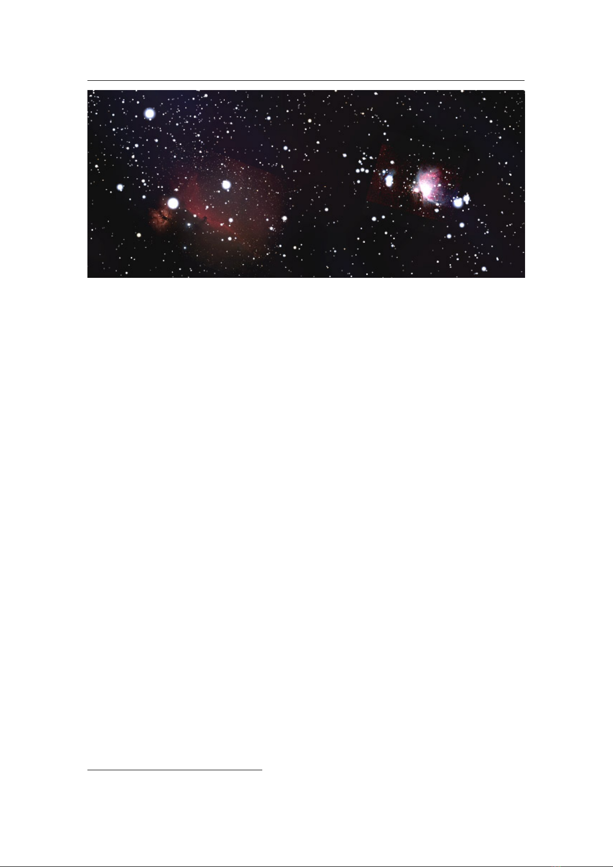
110 Chapter 9. Sky Cultures
The first line of the file starts with the only Level 1 header, i.e., a line starting with a single hash (
#
), a
space and then the name of the skyculture. This name is used in the selection list in the Sky Culture GUI
(see 4.4.6).
The other sections typically start with Level 2 or 3 headers (with two or three hash characters) which are
displayed as smaller section and subsection titles (HTML:
h2
or
h3
, respectively). All header lines (except
the first) should be enclosed by empty lines.
The continuous text should be formatted like that, please do not add newlines where they do not signal
the end of a paragraph with an empty line. Use an editor which just auto-wraps long lines to the window
width. These long lines/paragraphs are automatically fed into the translation system. References (see 9.1.2)
should be given like [#42].
You should provide a good description in the interest of future users: some cultural/ethnographical
background of the users of this sky culture, the history or background of sky culture research that provided
this work, tables of names/translations, links to external resources, whatever seems suitable. The length of
the description texts is not limited, but of course if this is your PhD thesis work, there is no need to repeat all
500 pages, you can add a link to the references.
The skyculture description should include the following Level 2 sections. Any other section must be a
subsection (i.e. Level 3 or deeper) of one of these sections. Each of these sections except
Constellations
will have its own entry in the translations files. The
Constellations
section will be split, so that each
constellation’s description will be translated separately.
Introduction – a summary that could ideally be shown on a small screen entirely.
Description – the actual text of the description.
Constellations
– a sequence of Level 5 sections, where the header is the
"english"
name of a constel-
lation (as given in the
index.json
file), and the body gives some information on this constellation.
This text is used for display and speech output when the constellation is selected.v 25.4
References – a list of references, see 9.1.2 for details.
Authors – all authors and acknowledgments go here.
License
– either a license id (see 9.1.3), or a sequence of lines separated by empty lines (i.e. Markdown
paragraphs) describing which part of the culture has which license, in the format "Sky culture item:
License-ID".
Note that the
Constellations
section has the strict format described above. In particular, there’s no
place for an introduction for all the constellations, or closing remarks or a similar deviation from the format
of this section. If this kind of text is desired, it can be placed in a subsection of the Description section.
To allow the correct display of special characters like ÄÖÜßáé you must provide the file in UTF-8
encoding. If you write only English/ASCII, this may not be relevant.
9.1.1 Images
You can also have embedded images in the file (your book cover? Views of sacred landscapes/buildings/art-
work/.. . ?), just provide them in PNG or JPG format please. Use the following syntax, where the last line is
fixed and is required for proper formatting.

My i mage captio n
{: . im g _ a n d _ c a p tion }
Alternatively, you can format an image in HTML if you need specialized extras like right-alignment or
size specifications:
<p >
<img src =" illustrations / my_im a g e . png " w idth =" 150 " align =" ri ght "/ >
My i mage captio n
{: . im g _ a n d _ c a p tion }
</p >
or (note the manual <br/>)
<p c lass =" img_and_capt i o n " >
<img src =" illustrations / my_im a g e . png " w idth =" 150 " align =" ri ght "/ > <br />
My i mage captio n
{: . im g _ a n d _ c a p tion }
</p >

9.1 Text descr iption 111
9.1.2 References
The optional Level 2 section “References” contains a list of information sources. Each line of the section
contains one record of 2 discernible fields: a hyphen followed by a numerical key in brackets, a colon and
then the actual description of the reference. The latter may include hyperlinks, e.g.:
- [# 1]: Kunitzsch , P .; Smart T. (2006) . " A D i c tionary of Moder n star Names : ...
This list is most important for “traditional” sky cultures collected from various sources to provide
traceable references.
Caution!
These reference numbers are not only used in the text, but also in the data description. If you re-arrange
references, you must also fix all affected references in the JSON file (9.2).
9.1.3 License
The level 2 section “License” is mandatory if you want your sky culture to be distributed with Stellarium to
prevent “unexpected” distribution of your content to other software or applications out of our hands.
We recommend to use one of the following possible licenses in this section:
GNU GPL v2.0 (or later)
– this is the most famous “copyleft” license for code and it may be acceptable
also for text and data.
CC0
(No Rights Reserved) – this is a “don’t care” license. Content may be freely distributed without
attribution for all purposes.
CC BY
(Creative Commons Attribution License) – this license lets others distribute, remix, adapt, and build
upon your work, even commercially, as long as they credit you for the original creation. This is the
most accommodating of licenses offered. Recommended for maximum dissemination and use of
licensed materials.
CC BY-SA
(Creative Commons Attribution-ShareAlike License) – this license lets others remix, adapt, and
build upon your work even for commercial purposes, as long as they credit you and license their new
creations under the identical terms. This license is often compared to “copyleft” free and open source
software licenses. All new works based on yours will carry the same license, so any derivatives will
also allow commercial use. This is the license used by Wikipedia, and is recommended for materials
that would benefit from incorporating content from Wikipedia and similarly licensed projects.
CC BY-ND
(Creative Commons Attribution-NoDerivatives License) – this license lets others reuse the
work for any purpose, including commercially; however, it cannot be shared with others in adapted
form, and credit must be provided to you.
CC BY-NC
(Creative Commons Attribution-NonCommercial License) – this license lets others remix, adapt,
and build upon your work non-commercially, and although their new works must also acknowledge
you and be non-commercial, they don’t have to license their derivative works on the same terms.
CC BY-NC-SA
(Creative Commons Attribution-NonCommercial-ShareAlike License) – this license lets
others remix, adapt, and build upon your work non-commercially, as long as they credit you and
license their new creations under the identical terms.
CC BY-NC-ND
(Creative Commons Attribution-NonCommercial-NoDerivatives License) – this license is
the most restrictive of the six main Creative Commons licenses, only allowing others to download
your works and share them with others as long as they credit you, but they can’t change them in any
way or use them commercially.
FAL
For illustrations we also expect usage of the Free Art License
1
(in addition to any other licenses) – it
is a “copyleft” license that grants the right to freely copy, distribute, and transform creative works.
You can specify, e.g., “GPL2, FAL” to indicate that the images are additionally released under Free
Art License.
Creative Commons provides a range of licenses
2
, each of which grants different rights to use the materials
licensed under them. All of these licenses offer more permissions than “all rights reserved”. Some of
Creative Commons are free and some are non-free. For example you can apply only the most permissive of
its licenses (CC0, CC BY and CC BY-SA) to material you create, to meets the Freedom Defined definition
of a “Free Cultural Work”.
3
1
https://artlibre.org/licence/lal/en/
2
Creative Commons License Chooser – https://creativecommons.org/choose/
3
See Creative Commons website to details –
https://creativecommons.org/share-your-work/public-d
omain/freeworks
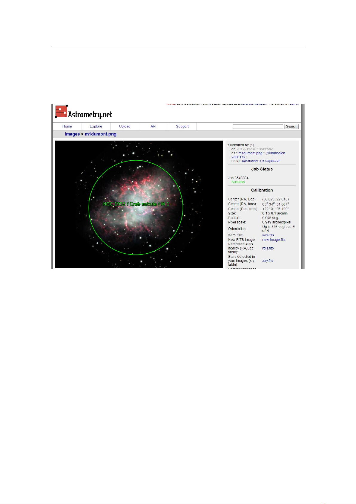
112 Chapter 9. Sky Cultures
If you have used one of the keys above in your
license
entry, a short (unofficial! Informative only)
description of license conditions will be displayed. You can use other licenses as well, but then please
describe the conditions sufficiently well in this section.
Caution for users!
While Stellarium is provided under the free GPL v2.0 licence which allows for commercial use, some of our
sky cultures have been contributed under CC NC/ND licenses, i.e., are for noncommercial use only. Please
respect their heritage holders and check the CC licence version in the description before you use sky cultures
in public events like TV documentaries, YouTube videos, lectures, planetarium shows or printed matter. If in
doubt, contact the respective authors.
9.1.4 Technical Test
Using correct syntax is required for making display and translation work. If you have checked out Stellarium’s
sources, you can run
util / skyculture s / generate - pot . py -s my_c ult ure
This may emit some warnings about issues that should be fixed (if any remain). It will also generate a
.po
directory in the skycultures directory, but these files aren’t supposed to be committed, you can remove it.
9.2 Technical data: index.json
The file
index.json
contains all “technical data” of the skyculture. JSON is a text-based format in which
strings, numerical values and arrays can be stored in nested dictionaries, i.e. unordered collections of comma-
separated
"tag": value
pairs in braces:
{ "Tag1": "Value1", "number": 123.456 }
. Values
can be strings, numbers, arrays or other dictionaries. Arrays are ordered sequences in
[...]
delimiters. You
must take care to close any open brackets and separate entries by commas.
{
" id " : " mode rn " ,
" regio n ": " World " ,
" cl a s s i f ication ": [ " traditional "] ,
" fallb a c k _ to _ i n t er n a t i on a l _ n am e s " : false ,
" as terisms ": [ ... ] ,
" co n s t e l lations ": [ ... ] ,
" ed g e s_type ": " iau " ,
" ed g e s _ s o u r c e " : " https :// p b arbier . com / co n s t e l l a t i o n s / edg e s _18 . txt " ,
" ed g e s _ e p och ": " B1 875 ",
" edges ": [ ... ] ,
" co m m o n _ n a m e s " : { ... }
}
in which
"id" A unique identifier for program-internal use. It is never displayed to users.
"region" See 9.2.1
"classification" See 9.2.2
"fallback_to_international_names"
if
true
, the IAU-approved star names are loaded after all names
given here, so names will be mixed without a clear separation, and newly-approved star names will
just appear automatically. Also all DSO names from
nebulae/default/names.dat
are loaded.
This is most useful for skycultures which have no names of their own, or where such mix is intended,
like
"personal"
contemporary skycultures (see 9.2.2) which are allowed to auto-adapt to newly
given names.
"common_names" includes names for star, planet and deep-sky objects, see 9.2.7
"constellations" describes constellations, see 9.2.4
"edges..." describes boundaries between constellations, see 9.2.3
"asterisms" describes asterisms, see 9.2.5
Tags not described here may be used in other programs but are ignored by Stellarium.
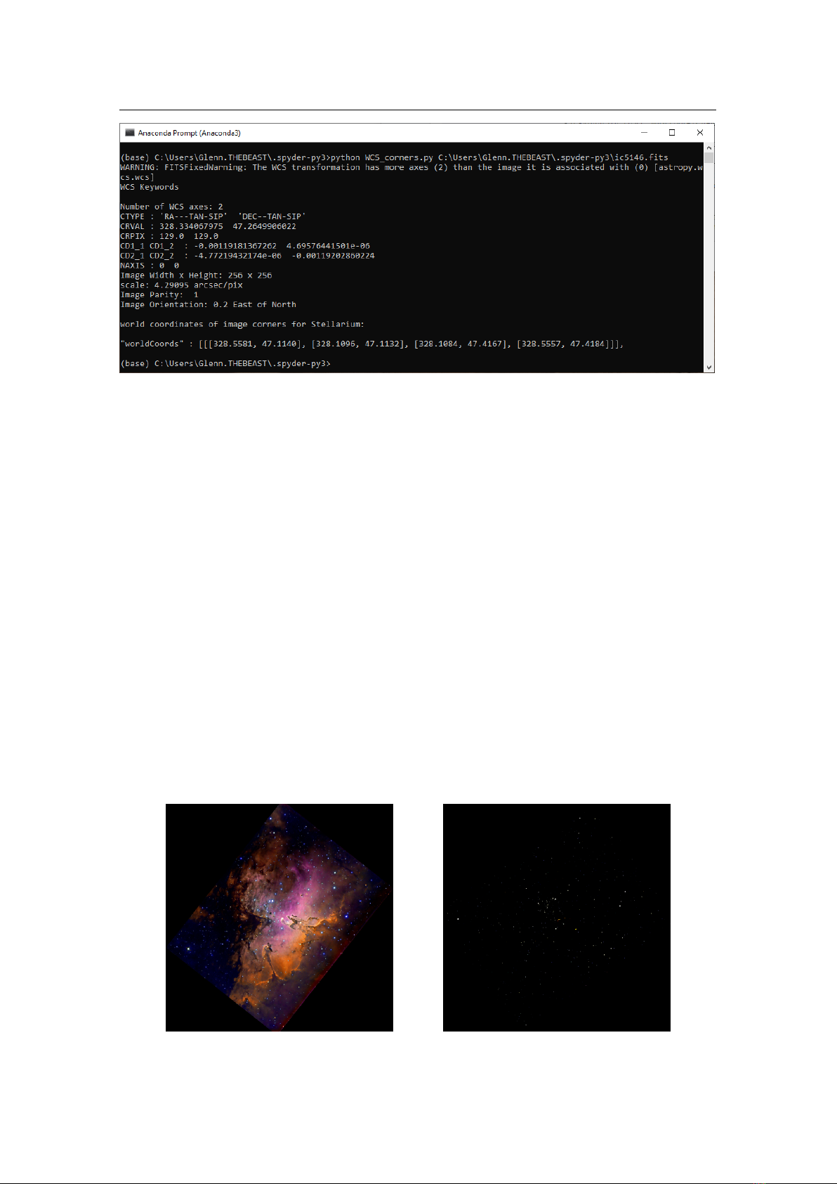
9.2 Technical data: index.json 113
9.2.1 Region
The “region” tag marks the origin region of the respective sky culture. It allows some form of additional
grouping. The names of regions are largely following the United Nations geoscheme UN M49
4
, but with
some deviations:
Northern Africa – Algeria, Egypt, Libya, Morocco, Sudan, Tunisia, Western Sahara.
Eastern Africa
– British Indian Ocean Territory, Burundi, Comoros, Djibouti, Eritrea, Ethiopia, French
Southern Territories, Kenya, Madagascar, Malawi, Mauritius, Mayotte, Mozambique, Réunion,
Rwanda, Seychelles, Somalia, South Sudan, Uganda, United Republic of Tanzania, Zambia, Zim-
babwe.
Central Africa
– Angola, Cameroon, Central African Republic, Chad, Congo, Democratic Republic of the
Congo, Equatorial Guinea, Gabon, Sao Tome and Principe.
Southern Africa – Botswana, Eswatini, Lesotho, Namibia, South Africa.
Western Africa
– Benin, Burkina Faso, Cabo Verde, Côte d’Ivoire, Gambia, Ghana, Guinea, Guinea-Bissau,
Liberia, Mali, Mauritania, Niger, Nigeria, Saint Helena, Senegal, Sierra Leone, Togo.
Caribbean
– Anguilla, Antigua and Barbuda, Aruba, Bahamas, Barbados, Bonaire, Sint Eustatius and Saba,
British Virgin Islands, Cayman Islands, Cuba, Curaçao, Dominica, Dominican Republic, Grenada,
Guadeloupe, Haiti, Jamaica, Martinique, Montserrat, Puerto Rico, Saint Barthélemy, Saint Kitts and
Nevis, Saint Lucia, Saint Martin (French Part), Saint Vincent and the Grenadines, Sint Maarten (Dutch
part), Trinidad and Tobago, Turks and Caicos Islands, United States Virgin Islands.
Central America – Belize, Costa Rica, El Salvador, Guatemala, Honduras, Mexico, Nicaragua, Panama.
South America
– Argentina, Bolivia (Plurinational State of), Bouvet Island, Brazil, Chile, Colombia,
Ecuador, Falkland Islands (Malvinas), French Guiana, Guyana, Paraguay, Peru, South Georgia and
the South Sandwich Islands, Suriname, Uruguay, Venezuela (Bolivarian Republic of).
Northern America – Bermuda, Canada, Greenland, Saint Pierre and Miquelon, United States of America.
Antarctica – Antarctica.
Northern Asia – Russian Federation (Asian part).
Central Asia – Kazakhstan, Kyrgyzstan, Tajikistan, Turkmenistan, Uzbekistan.
Eastern Asia
– China, Hong Kong Special Administrative Region of China, Macao Special Administrative
Region of China, Democratic People’s Republic of Korea, Japan, Mongolia, Republic of Korea,
Taiwan.
South-eastern Asia
– Brunei Darussalam, Cambodia, Indonesia, Lao People’s Democratic Republic,
Malaysia, Myanmar, Philippines, Singapore, Thailand, Timor-Leste, Viet Nam.
Southern Asia
– Afghanistan, Bangladesh, Bhutan, India, Iran (Islamic Republic of), Maldives, Nepal,
Pakistan, Sri Lanka.
Western Asia
– Armenia, Azerbaijan, Bahrain, Cyprus, Georgia, Iraq, Israel, Jordan, Kuwait, Lebanon,
Oman, Qatar, Saudi Arabia, State of Palestine, Syrian Arab Republic, Türkiye, United Arab Emirates,
Yemen.
Eastern Europe
– Belarus, Bulgaria, Czechia, Hungary, Poland, Republic of Moldova, Romania, Russian
Federation (European part), Slovakia, Ukraine.
Northern Europe
– Åland Islands, Channel Islands, Denmark, Estonia, Faroe Islands, Finland, Iceland,
Ireland, Isle of Man, Latvia, Lithuania, Norway, Svalbard and Jan Mayen Islands, Sweden, United
Kingdom of Great Britain and Northern Ireland.
Southern Europe
– Albania, Andorra, Bosnia and Herzegovina, Croatia, Gibraltar, Greece, Holy See, Italy,
Malta, Montenegro, North Macedonia, Portugal, San Marino, Serbia, Slovenia, Spain.
Western Europe
– Austria, Belgium, France, Germany, Liechtenstein, Luxembourg, Monaco, Netherlands,
Switzerland.
Australasia
– Australia, Christmas Island, Cocos (Keeling) Islands, Heard Island and McDonald Islands,
New Zealand, Norfolk Island.
Melanesia – Fiji, New Caledonia, Papua New Guinea, Solomon Islands, Vanuatu.
Micronesia
– Guam, Kiribati, Marshall Islands, Micronesia (Federated States of), Nauru, Northern Mariana
Islands, Palau, United States Minor Outlying Islands.
Polynesia
– American Samoa, Cook Islands, French Polynesia, Niue, Pitcairn, Samoa, Tokelau, Tonga,
Tuvalu, Wallis and Futuna Islands.
For “modern” sky cultures we use the special region name World to define worldwide applicable data.
4
Standard country or area codes for statistical use (M49) – https://unstats.un.org/unsd/methodology/m4
9/
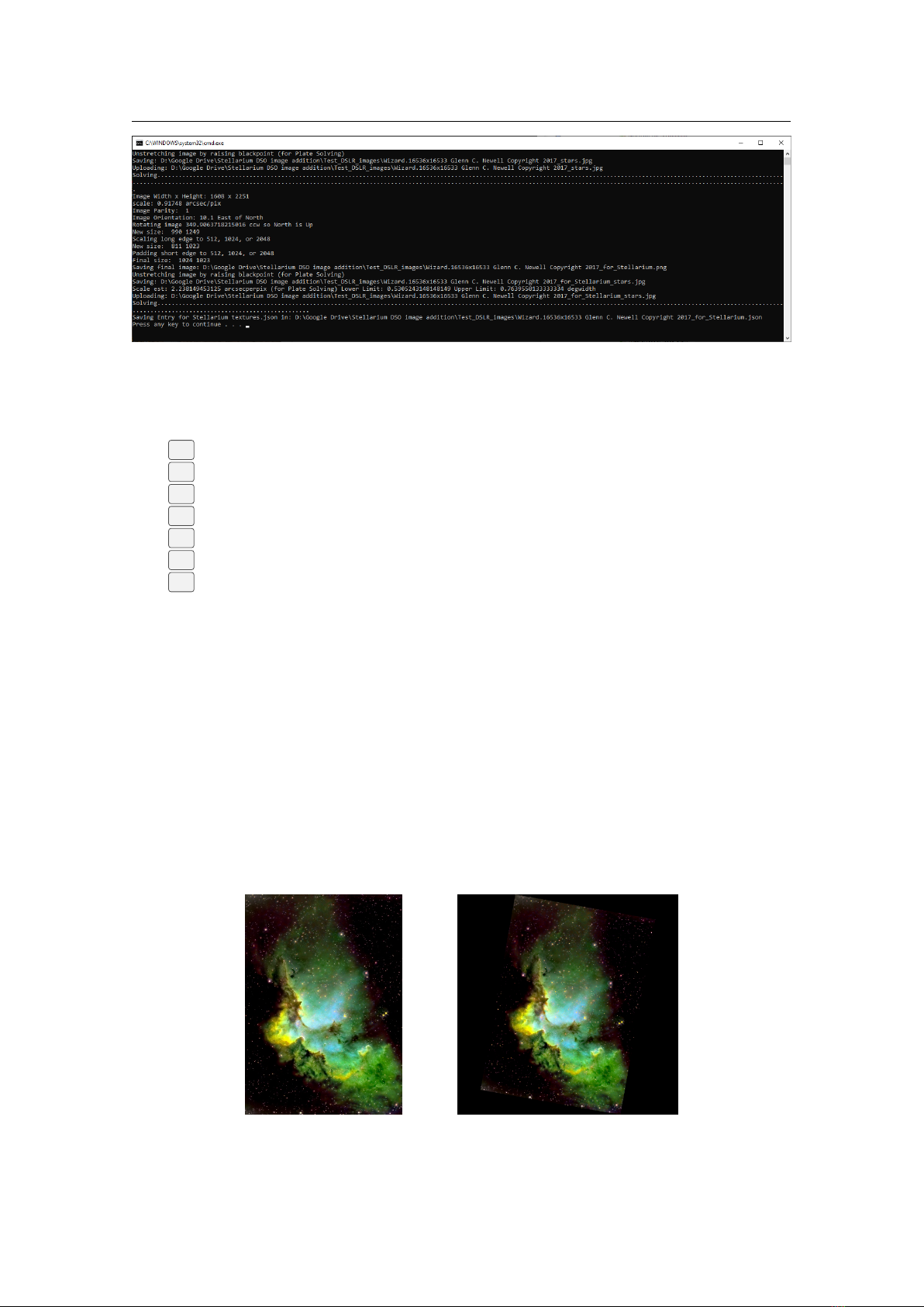
114 Chapter 9. Sky Cultures
In case you are illustrating a fictional sky culture not actually used on Earth, you can use Other or even
whatever else you like. They will be listed in the “Other” category in the View dialog.
Figure 9.1: Africa: subregions as delineated by United Nations geographic classification scheme:
Eastern Africa, Central Africa, Northern Africa, Southern Africa, Western Africa.
Wikipedia / CC BY-SA 3.0
9.2.2 Classification
The tag “classification” allows describing the origin and intended use of this skyculture:
personal
– this is a personally developed sky culture which is not founded in published historical or
ethnological research. Stellarium may include it when it is “pretty enough” without really approving
its contents.
traditional
– (default value) content represents “common” knowledge by several members of an ethnic
community, and the sky culture has been developed by members of such community. Our “Modern”
sky culture is a key example: rooted in antiquity it has evolved for about 2500 years in what is now
commonly known as “western” world, and modern astronomers use it.
ethnographic – provided by ethnographic researchers based on interviews of indigenous people.
historical – based on historical written sources from a (usually short) period of the past.
single – represents a single source like a historical atlas, or related publications of a single author.
comparative
– special-purpose compositions of e.g. artwork from one and stick figures from another sky
culture, and optionally asterisms as representations of a third. Or comparison of two stick figure sets
in constellations and asterisms. These figures sometimes will appear not to fit together well. This may
be intended, to explain and highlight just those differences! The description text must clearly explain
and identify all sources and how these differences should be interpreted.
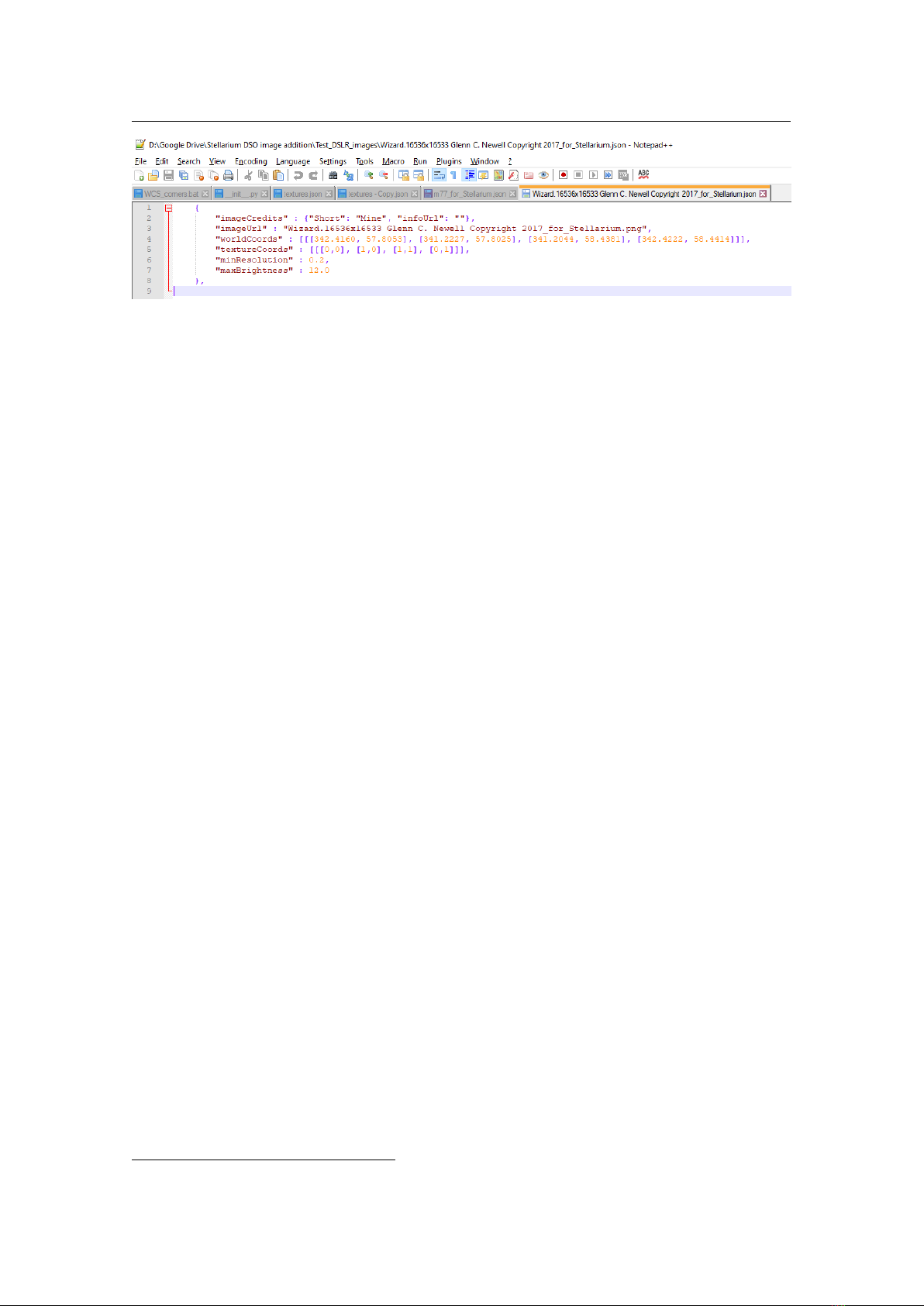
9.2 Technical data: index.json 115
Figure 9.2: Asia: subregions as delineated by United Nations geographic classification scheme:
Central Asia, Eastern Asia, South-eastern Asia, Southern Asia, Western Asia,
Northern Asia. Wikipedia / CC BY-SA 3.0
Figure 9.3: Europe: subregions as delineated by United Nations geographic classification scheme:
Eastern Europe, Northern Europe, Southern Europe, Western Europe. Wikipedia / CC
BY-SA 3.0

116 Chapter 9. Sky Cultures
Figure 9.4: Americas: subregions as delineated by United Nations geographic classification scheme:
Caribbean, Central America, Northern America, Southern America. Wikipedia / CC
BY-SA 3.0
Figure 9.5: Oceania: subregions as delineated by United Nations geographic classification scheme:
Australasia, Melanesia, Micronesia, Polynesia. Wikipedia / CC BY-SA 3.0
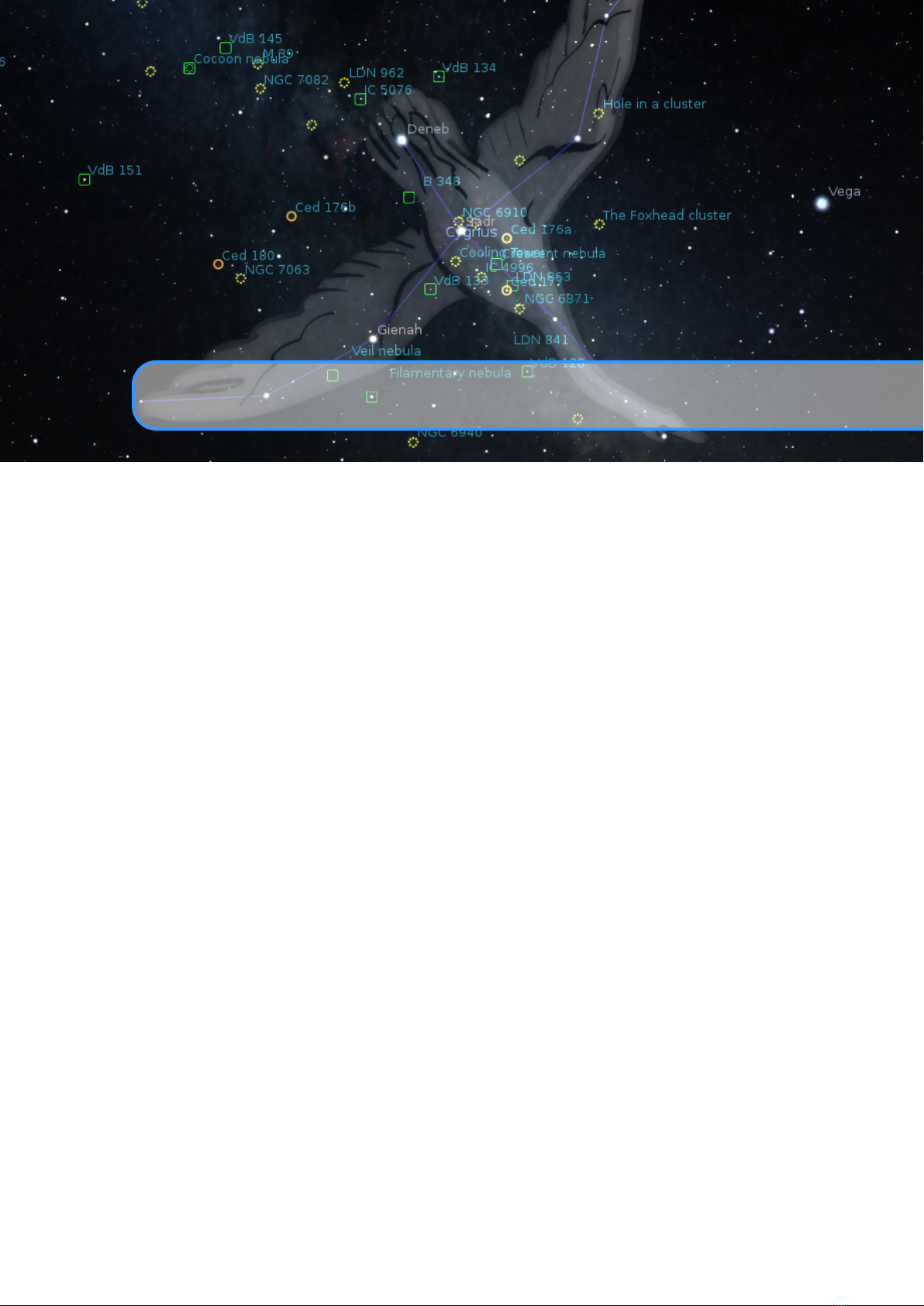
9.2 Technical data: index.json 117
9.2.3 Constellation boundaries
In the late 18th century, when variable stars started to be catalogued by a code that included the star’s
constellation, a necessity arose to define which sky region belonged to which constellation. Atlases of
this period showed curved boundaries between the constellations. Such boundaries are hard to describe
by coordinates, though. The Uranographia Argentina (Gould, 1879) proposed a different approach. The
boundaries were described by mostly straight segments along great circles of equal right ascension and small
circles of equal declination. The atlas used coordinates for epoch B1875.0. Based on this work, in 1930
the International Astronomical Union (IAU) ratified a partition of the sky into the 88 constellations (now
only using lines along constant right ascension/declination of B1875.0) used by scientists and amateurs ever
since. When looking at these boundaries in J2000.0 coordinates, we can see they are no longer parallel to the
J2000.0 coordinate grid, the deviation caused by precession.
Partitions of the full sky into contiguous regions defined by edges between coordinate vertices defined in
equatorial coordinates at a certain epoch can be described in the following elements of the index.json:
" ed g e s_type ": " iau " ,
" ed g e s _ s o u r c e " : " https :// p b arbier . com / co n s t e l l a t i o n s / edg e s _18 . txt " ,
" ed g e s _ e p och ": " B1 875 ",
" edges ": [
" 001:00 2 M + 2 2:52:00 +34 : 3 0 :00 22:52:0 0 +52:30:00 AND LAC " ,
" 002:00 3 P + 2 2:52:00 +52 : 3 0 :00 23:20:0 0 +52:30:00 AND CAS " ,
" 004:00 5 P + 2 3:20:00 +50 : 0 0 :00 23:35:0 0 +50:00:00 AND CAS " ,
...
]
where
"edges_type" is optional and may contain the following values:
"none"
— (default) designates that this culture doesn’t have constellation boundaries, and any
edges
entry is ignored.
"iau" — use this value for variants of “modern” sky cultures to declare use of IAU boundaries.
"own" — used for cultures which have their own set of constellation boundaries.
"edges_source" is optional and only given for reference. It is not evaluated.
"edges_epoch" describes the coordinate epoch. Allowed values:
"J2000" (default)
"B1875" used for the edge list defining the IAU borders.
"Byyyy.y" (a number with B prepended) Arbitrary epoch as Besselian year.
"Jyyyy.y" (a number with J prepended) Arbitrary epoch as Julian year.
"JDddddddd.ddd" (a number with JD prepended) Arbitrary epoch as Julian Day number.
"ddddddd.ddd" (a pure number) Arbitrary epoch as Julian Day number.
The lines in the array “edges” were taken from the given reference. The first component is ignored. The
next element provides information whether the segment runs along a meridian (
M
, right ascension) or parallel
(
P
, declination) circle in ascending
+
or descending
-
sense. Then it provides
α
1
,
δ
1
,
α
2
,
δ
2
in sexagesimal
numbers (
α
in HH:MM:SS,
δ
in DD:MM:SS format) and the uppercased constellation abbreviations. As
described in the original source file, Serpens has been split into
SER1
and
SER2
, these tags are treated both
as SER.
These edges are used to define isolated boundaries for each constellation (for proper working of the
Select single constellation
option).
9.2.4 Constellations
Constellations are coded as array of dictionaries:
" co n s t e l lations ": [
{
" id " : " CON mode rn Aql ",
" lines ": [ [ 9 80 3 6 , 9 76 4 9, 9727 8 ] , [ 97 6 4 9, 9550 1 , 9 7 80 4 ], [9 94 7 3, 9780 4 ] ,
[95 5 0 1, 9374 7 , 9 3 24 4 ], [9 55 0 1, 9380 5 ] ],
" image ": {
" file ": " il l u s t r a t i o n s / aqu ila . png " ,
" size ": [5 1 2 , 5 12 ] ,
" anchor s " : [
{" pos ": [1 6 3 , 2 32 ] , " hip ": 9 7 6 49 } ,
{" pos ": [3 8 5 , 1 31 ] , " hip ": 9 3 2 44 } ,
{" pos ": [3 9 7 , 3 97 ] , " hip ": 9 3 8 05 }

118 Chapter 9. Sky Cultures
]
} ,
" co m m o n _ n ame ": { " engli sh ": " Aq uila ", " nativ e ": " Aq uila "}
} , ...
] , ...
where
"id"
A unique figure identifier, consisting of
CON
(for constellations), skyculture id, and a short Latin-
character based label still unique within the skyculture. For IAU-based skycultures, these short
labels must be the IAU standard labels. For others, you can invent your own. It is not necessary
to have exactly 3-letter keys, but they should act as mnemonic support, so numerical keys are not
recommended: the short label is displayed when enabling abbreviated screen labels (s. 4.4.6). If you
want to prevent certain abbreviations from being displayed, let them start with a dot. See the effect in
the
Modern (H.A.Rey)
sky culture: with abbreviated labels enabled, only the official abbreviations
are displayed.
"lines"
an array of arrays, each describing a polyline with star numbers. The star numbers are usually the
Hipparcos (HIP) numbers. For very dim stars, the longer numbers from the Gaia DR3 catalog are
acceptable, but they must be written as string. Even Deep-Sky objects (like a naked-eye open cluster)
v 25.2
can be added to a constellation line when written as string starting with "DSO:", like "DSO:M7".
To describe dark constellations formed from dust clouds in the Milky Way or other non-stellar items,
v 25.2
another variant can use coordinate lists and is technically an array of arrays of 2-part arrays of float
numbers, each pair being right ascension
α
(decimal hours) and declination
δ
(decimal degrees) in
equinox J2000.0. See below how Stellarium can help you write these arrays.
Single-star constellations or particular highlights can be described with just one star repeated in a
v 25.1
two-element segment. The respective star will be encircled with a radius of
"single_star_radius" (float, default 0.5).v 25.1
"hull_extension"
(optional) A vector of star IDs (HIP number as integer, Gaia DR3 long integer
v 25.2
number as string, or a Deep-Sky object (like a naked-eye cluster) as string starting with
"DSO:"
, like
"DSO:M44" that are seen as part of the constellation. See below about convex hull.
"hull_radius" (float, defaults to "single_star_radius" or (if that is not defined)0.5).v 25.2
"image" Optional, see 9.2.4.1
"common_name" Dictionary of names.
"native" name in the original language of the skyculture.
"english" translation of the name’s meaning. This is translated to users’ language.
"byname"
an optional explanatory addition to the name. May be helpful to explain mythological
v 25.3
figures. This is translated to users’ language, but is not included in search functions.
"pronounce"
(optional, but recommended) a Latin-character based transliteration/pronunciation
aid, e.g. Pinyin for Chinese. This may also be translated to user language.
"transliteration"
(optional) a scientific Latin-character based transliteration where applicable.
This is not translatable or adaptable to user language conventions, but may include extended
diacritics. An example is Wylie for Tibetan, which is not meant to help in pronunciation.
"IPA" (optional) International Phonetic Alphabet, a standardardized phonetic spelling.
"context"
(optional) Short english explanation that helps to disambiguate terminology. Not dis-
played in the program.
"translators_comments"
(optional) English explanations that help in translation on Transifex.
Not displayed in the program.
These names are used in the sky culture name style settings (s. 4.4.6). If your sky culture is a variant
of the
Modern
sky culture, please use the canonical Latin as
"native"
name and the
"english"
names from the default Modern skyculture, they have all been translated already. Also star names
should provide both
"native"
and
"english"
entries, even if both are identical, to allow transla-
tion/transliteration to languages with other script systems or spelling variants.
If your sky culture is not a variant of the generally known
Modern
(western) sky culture, please
make sure to provide an
"english"
translation (where possible) in addition to the name given in the
"native"
language, or a
"byname"
which may help better understanding a figure. Else translators
will not be able to translate the name, and users will be less interested to learn about the culture. Also
make very sure to use the same spelling consistently in
index.json
and
description.md
, and
explain the context of stars (how these stars are used, or what they mean to the respective members of
the culture), especially where only an untranslatable proper name is given.

9.2 Technical data: index.json 119
"label_offset"
optional. An array of
[deltaRA, deltaDE]
(decimal degrees) used as offset that shifts
the auto-computed label positions.
"label_positions"
optional. An array of sub-arrays of
[RA, DE]
tuples (decimal hours, decimal
degrees) used as label positions. By default, the label position is computed from the star positions
used in the
"lines"
. With this entry you can set specialized positions, or also use more than one
label per constellation.
"visibility"
(optional) special cases for rule-based visibility, e.g. seasonally changing aspects of figures.
Currently only a
"months"
rule has been defined. Its “payload” is an array of two integers, start and
end of visibility in months, e.g:
" visi bility ": { " months ": [ 6 , 3 ]} ,
This specifies that the afflicted constellation is visible only from June to March, wrapping over the
12-month cycle. A second entry of the same constellation (with possibly different lines, artwork, or
even name) that would be visible from April to May, would be specified as:
" visi bility ": { " months ": [ 4 , 5 ]} ,
Drawing dark constellations
The outlines of figures like the “Emu in the Sky” cannot be described with connect-the-dot star patterns, as
v 25.2
they are formed from the absence of luminous patterns. We need to describe them using coordinate lists. To
make the process less tedious, we can extend setting Markers (see 3.6). For this to work, add the following
key to config.ini:
[ devel ]
ma rkers _t o_log file = true
After program restart, setting a marker also writes a numbered line into the logfile, containing marker number
and the array of coordinates (
[RA, dec]
). In the text editor you are using to edit
index.json
, the arrays
can be collated into the format required to code coordinate lists for dark constellations.
Constellation area (convex hull)
The constellation area, or convex hull of a constellation, is an area of the sky described by a convex polygon
v 25.2
which surrounds all stars that are part of the lines that form the constellation “stick figure”, plus those
objects which are listed in
"hull_extension"
. While the IAU has defined 88 constellation areas in 1930,
constellations of other cultures are not as clearly defined. These areas can help analyzing historical records.
Note that a point may lie in zero, one or more than one constellation area(s) when it overlaps two or even
more adjacent figures.
Technically, the stars are projected perspectively onto a tangential plane to the celestial sphere at the
balance point of all involved stars. Then a simple package wrapping algorithm (Sedgewick, 1990, ch.25)
can be applied to find the convex hull. Straight lines in the projection are great circle arcs. Note that this
limits constellation size to less than 180 degrees in the sky, outlying stars will currently be discarded. (Please
report an error if this affects you, so we might find a better solution.)
This functionality is an advanced topic mostly used by sky culture researchers (e.g. S. M. Hoffmann,
2017, pages 94–98) who are also not afraid of calling scripting functions (see ch. 17), and is therefore hidden
from beginning users. To make use of it, edit your config.ini and add a key:
[ gui ]
sk yc ulture_ enable_ hu lls = true
The constellation areas of a skyculture can be queried by a scripting function:
ConstellationMgr.outputHullAreas(<filename_start>);
The argument
<filename_start>
is optional and defaults to
"hullAreas"
. The created CSV file
<filename_start>_skycultureName.csv
in your Stellarium user data directory lists hull areas for
all constellations of the current skyculture.
You can list stars which belong to a thusly defined constellation with a scripting function:
ConstellationMgr.starsInHullOf("Taurus", false, 12.0, <start>);

120 Chapter 9. Sky Cultures
This creates a file
hullStars_Modern_Taurus-12.00.csv
in your Stellarium user data directory which
contains all stars within the convex hull of Taurus in the current (here: “Modern”) sky culture. The arguments
to the function are:
constellation string; name or abbreviation.
hipOnly
Boolean, optional, defaults to
true
; if you are only interested in brighter stars contained in the
Hipparcos catalog, set it true.
maxMag
float, optional, default: 25.0. Dimmest stellar magnitude to use. The default value just makes sure
all stars that are contained in the catalogs are listed, the result will only have few entries dimmer than
mag 18.
<start> string, optional, default hullStars; the start of the filename can be changed here.
9.2.4.1 Constellation Artwork
Constellation artwork is optional, but may give your sky culture the final touch, if it requires artwork at all.
E.g., H. A. Rey’s variant of the
Modern
sky culture deliberately does not contain artwork other than his new
set of stick figures.
Each constellation artwork is linked to 3 stars in its constellation. This is programmed in the
"image"
dictionary. It contains entries
"file"
is the file name of your texture. All constellation artwork files should reside in a subdirectory
illustrations
. For best efficiency it should be sized in a power of two, like
512× 512
,
1024× 2048
etc. Avoid dimensions larger than 2048, they are not supported on all systems. Use as little border in
your textures as possible instead. You can distort images to better exploit the pixels, the texture will
be stretched back. The background of the artwork image must be absolutely black.
"size"
Image size (width, height) in pixels. This size specified here, and not the real image size, is relevant
for the
"anchors"
entry. This may be important on very memory limited systems where you decide
to downscale all textures.
"anchors" An array of three similar dicts with
"pos" pixel addresses [x, y] given from upper left corner (find those in any image editor)
"hip"
The star index as Hipparcos (HIP) number, given as integer. This may technically also be a
Gaia DR3 number when given as string.
In case the artwork is only available in a certain projection (e.g., an all-sky map), or is otherwise heavily
distorted so that the match is not satisfactory, you may have to re-project the image somehow. For aligning,
you should switch Stellarium to Stereographic projection for optimal results.
You don’t have to shutdown and restart Stellarium during creation/matching, you can just press
Ctrl
+
Alt
+
I
to reload.
9.2.5 Asterisms and help rays
Sometimes auxiliary figures were created for easier orientation. Some part of a constellation may have
been redefined into a figure in its own right, or parts from different constellations were merged into one big
figure — e.g. “Big Dipper” as part of Ursa Major, or the “Summer Triangle” consisting of 3 stars from the
constellations Cygnus, Lyra and Aquila. After the codification of the official 88 constellations by the IAU,
those additional figures have generally been called asterisms.
5
Other simple figures might be used as navigation and orientation helpers: the help rays. As example
to help in orientation in the sky the additional lines between constellations Ursa Major, Ursa Minor and
Cassiopeia might be useful. The asterisms and help rays are listed in
"asterisms"
which is similar to the
"constellations" dict, but has no "figures" entry:
" as terisms ": [
{
" id " : " AST mode rn HeG ",
" co m m o n _ n ame ": { " engli sh ": " Heav e nly G " , " references ": [30 ,32 ] } ,
" lines ": [ [ 2 14 2 1 , 2 46 0 8, 3685 0 , 3 7 82 6 , 3 7 27 9 , 3 23 4 9 , 2 44 3 6, 2533 6 , 2 7 98 9 ] ]
} , ...
]
"id"
A unique asterism identifier, consisting of
AST
(for asterism), skyculture id, and a short Latin-character
based label still unique within the skyculture. It is not necessary to have exactly 3-letter keys, but they
should act as mnemonic support, so numerical keys are not recommended: the short label is displayed
5
In a more generalized context when describing the sky of other cultures, the distinction may be less strict, and the
term “asterism” may even be used for the “primary figures” observed by those cultures.

9.2 Technical data: index.json 121
when activating abbbreviated labels (s. 4.4.6). If you want to prevent certain abbreviations from being
displayed at all, let them start with a dot.
"common_name"
Another dict with entries
"native"
(as used in the source),
"english"
(the trans-
latable english name),
"pronounce"
,
"transliteration"
,
"IPA"
,
"byname"
,
"context"
and
"translators_comments"
as defined for constellations, and an optional array
"references"
which lists from which sources (from 9.1.2) this asterism was taken.
Collecting sources and giving such references is always a good idea. If you feel ther are more in the
collection than you like, read 9.2.9.1 about suppressing excessive entries.
"label_offset"
optional. An array of
[deltaRA, deltaDE]
(decimal degrees) used as offset that shifts
the auto-computed label positions.
"label_positions"
optional. An array of sub-arrays of
[RA, DE]
tuples (decimal hours, decimal
degrees) used as label positions. By default, the label position is computed from the star positions
used in the
"lines"
. With this entry you can set specialized positions, or also use more than one
label per asterism.
"is_ray_helper"
(optional, default=
false
). Set to
true
to declare this asterism as “ray helper” which is
shown in a different color and without label.
"lines"
an array of arrays, each describing a polygon with integer star numbers. The star numbers are
usually the Hipparcos (HIP) numbers. For the very dim stars of telescopic asterisms, the longer
numbers from the Gaia DR3 catalog are acceptable, but they must be written as string. Another variant
can use coordinate lists and is technically an array of arrays of 2-part arrays of float numbers, each
pair being right ascension
α
(decimal hours) and declination
δ
(decimal degrees) in equinox J2000.0.
Single-star asterisms can be described with a two-element array that repeats the first entry (star or
v 25.1
coordinate pair) – the respective star/coordinate will be encircled with a radius of
"single_star_radius"
(float, default 0.5) radius of a circle (degrees) marking single-star segments in
v 25.1
"lines".
9.2.6 Culture Relevant Coordinate Systems: Zodiac and Lunar Systems
Ancient high cultures in and around Asia took special note of the zone where the planets move: along the
v 25.2
path of the Moon, a system of 27 or 28 lunar stations or lunar mansions were formed, and later the Sun’s
annual path was split into 12 equal-size parts of 30 degrees along the ecliptic.
The best-known system in modern times is that of the tropical zodiac of
12× 30
degrees along the ecliptic,
counted from the equinox point (First point of Aries
à
). The 12 sections, or zodiacal signs, were named
after the constellations which resided there at the time the system was codified. Precessional movement
since antiquity moved the stars eastwards along the ecliptic by about one full sign, so that meanwhile
there is usually a mismatch between the constellation the sun is in and the sign which you find listed in
bad newspapers’ horoscope pages. Astronomically, the zodiacal sign is just an old-fashioned way to write
ecliptical coordinates of date.
In India, the partitions were defined so that the star Spica rests at the 180° mark, so that the Indian or
sidereal zodiac moves along the ecliptic with precession.
" zodia c ": {
" name ": { " pr o n o unce ": "R¯aśi" , " english " : " Indi an Zod iac "} ,
" contex t " : " ind ian zod iac sign " ,
" pa r t itions ": [ 1 2 , 3 , 2 , 5 ] ,
" exten t ": 9 ,
" link ": { " star ": 6 5 4 74 , " of fset ": 180} ,
" names ": [ { " sym bol ": "\ u2648 " , " native " : " ... " , " engli s h ": " Ram "} ,
{ " symbol " : " \u26 49 " , " native " : " ... " , " engli sh ": " Bull "} ,
...
{ " symbol " : " \u26 53 " , " native " : " ... " , " engli sh ": " Fi shes "} ]} ,
where
"name" cultural name as described in 9.2.7.
"context"
(optional, recommended) context data for all English names in zodiac (enhancement of local-
ization support).
"comment" (optional) commentary for zodiac, it will be used as extra commentary for translators also.
"partitions"
regular division of the centerline. The first element commonly is 12 (30-degree sign). The
other elements (up to 3) are used to describe the tick marks in decreasing order. The example means,
the 30 degrees are further divided in 3 sections (large 10-degree ticks), these are split in 2 5-degree
sections with 5 sections (1-degrees) each.
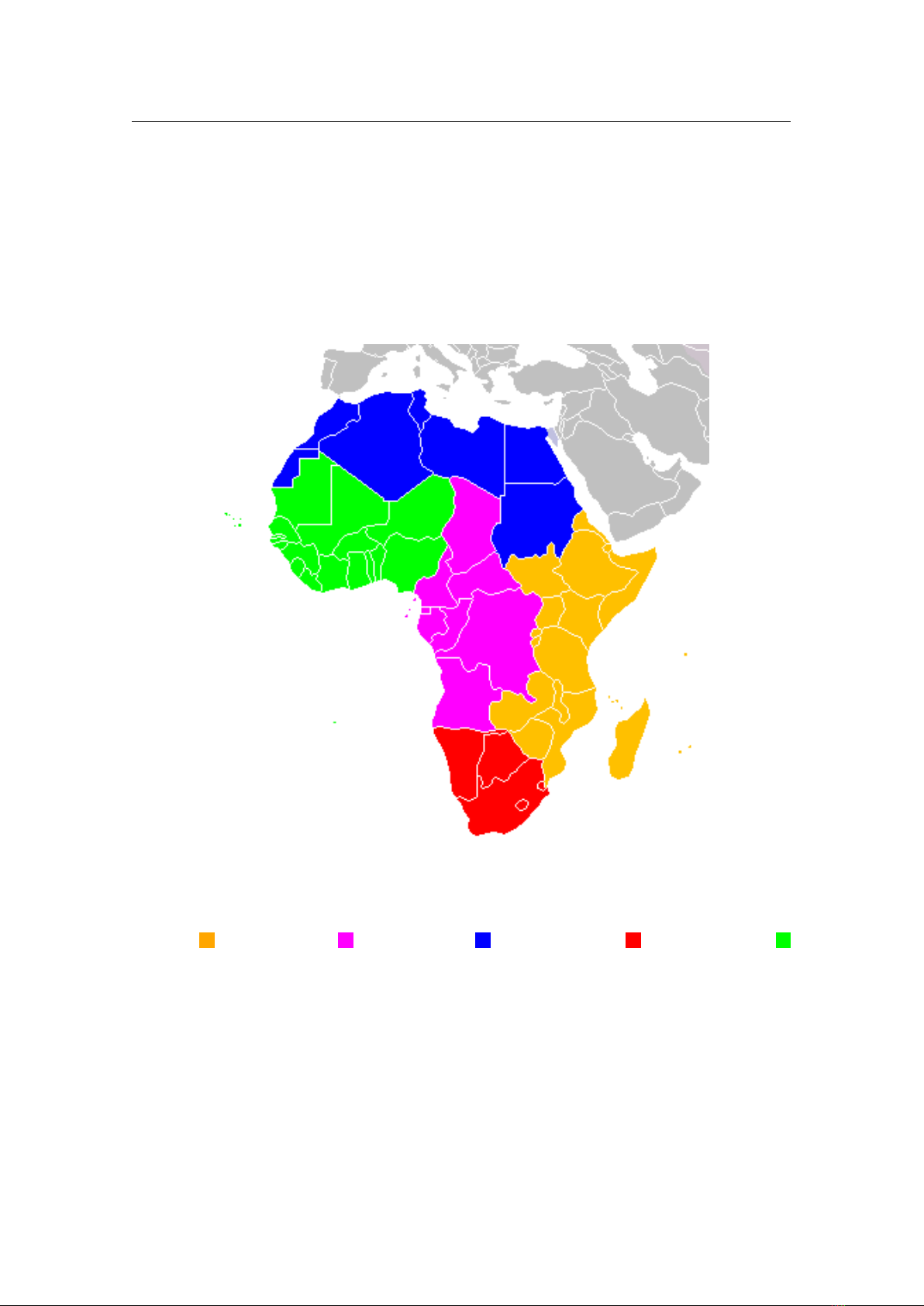
122 Chapter 9. Sky Cultures
"extent"
The zone of interest is closed off by parallel lines this many degrees north and south of the
centerline. A zodiac of 9 degrees encloses extreme positions of all major planets.
"link"
(optional) The Indian sidereal zodiac is described to be defined with the longitude of a certain star.
Usually and in this sample, Spica (
α
Vir, HIP 65474) is declared to lie at 180°. If missing, the zodiac
starts from à.
"names"
Sequence of names. In addition to the elements listed in 9.2.7,
"symbol"
provides a Unicode
symbol (as shown here, these are the common zodiacal signs) or 1-2 letter string (for practical reasons,
a number seems generally useful). The number of entries must be equal to (or larger than) the first
element of "partitions". Excessive entries are ignored.
More important for Indians however, and still relevant today, is the traditional system of lunar stations, the
nakshatras. the ecliptic is split into 27 equal-sized partitions, which are then further split into 4 equal parts.
" lu n a r _ s y s t e m " : {
" name ": { " native " : " ... ", ... , " engl i sh ": " Naksha t r a s " } ,
" contex t " : " ind ian lu nar ma nsion ",
" pa r t itions ": [ 2 7 , 4 ],
" exten t ": 5 ,
" link ": { " star ": 6 5 4 74 , " of fset ": 180} ,
" names ": [ { " sym bol ": "1 " , " nat ive ": " ... " , ... , " eng lish ": " Ph y s ician to the
↪ Gods "} ,
{ " symbol " : " 2" , " na tive ": " ... ", ... , " engli s h ": " Bea rer "} ,
{ " symbol " : " 3" , " na tive ": " ... ", ... , " engli s h ": " Plei a d es "} ,
...
where
"name" cultural name as described in 9.2.7.
"context"
(optional, recommended) context data for all English names in lunar mansions (enhancement
of localization support).
"comment"
(optional) commentary for lunar system, it will be used as extra commentary for translators
also.
"partitions" regular division of the centerline. 27 stations which are further divided in 4 equal parts.
"extent"
The zone of interest. With an obliquity of the Lunar orbit of about 5 degrees, a 5-degree zone
seems appropriate.
"link"
(optional) The Indian system is again described to be defined with the longitude of Spica (
α
Vir,
HIP 65474) to lie at 180°. If missing, the count starts from à.
"names"
Sequence of names. In addition to the elements listed in 9.2.7,
"symbol"
provides a Unicode
symbol or 1-2 letter string (for practical reasons, a sequential number seems generally useful). The
number of entries must be equal to (or larger than) the first element of
"partitions"
. Excessive
entries are ignored.
In the Arabian peninsula, a similar system of 28 lunar stations is in use until today, but the actual asterism
appears to be more important than the regularity of the ecliptic partition. The first station is centered around
al-Thurayya (the Pleiades star cluster). In some skycultures the “band” of stations around the ecliptic is
shown irregular, with boxes trying to frame the associated asterisms:
" lu n a r _ s y s t e m " : {
" name ": {" en glish ": " Lun ar Stati o ns " , " na tive ": " ... " , " pron o u n ce ": " Man a zil
↪ alQamar " , " IPA ": " manazilulqamar "} ,
" pa r t itions ": [ 2 8 , 3 , 2 ] ,
" exten t ": [ 1 0. 0 , -1 0 .0 , 1 0 .0 , - 1 0 .0 , 1 0 .0 , - 1 5 .0 , 1 0 .0 , - 1 5 .0 , 1 5 .0 , ... ] ,
" contex t " : " arab i an lun ar stat i o ns " ,
" link ": { " star ": 1 7 7 02 , " of fset ": 6.42 8 5 71 4 28 5 71 4 2 9, " comme n t ": " ce nter of
↪ f irst s tation is Lucida P l eiadum "} ,
" names ": [ { " sym bol ": " 1" , " eng lish ": "Al - Th urayya ", " nativ e ": " ... " , ... } ,
{ " symbol " : "2 " , " eng l ish ": " Al - Da baran " , " nati ve ": " ... ", ... } ,
...
where
"partitions"
regular division of the centerline. 28 stations which are further divided into 3 equal parts
that are further halved.
"extent"
As array of latitude coordinates, they provide alternating north and south latitudes for all stations.
v 25.3
The number of entries must be twice the number of partitions.
In China, the 28 lunar mansions are defined in a different way. 28 defining stars mark the begin (western
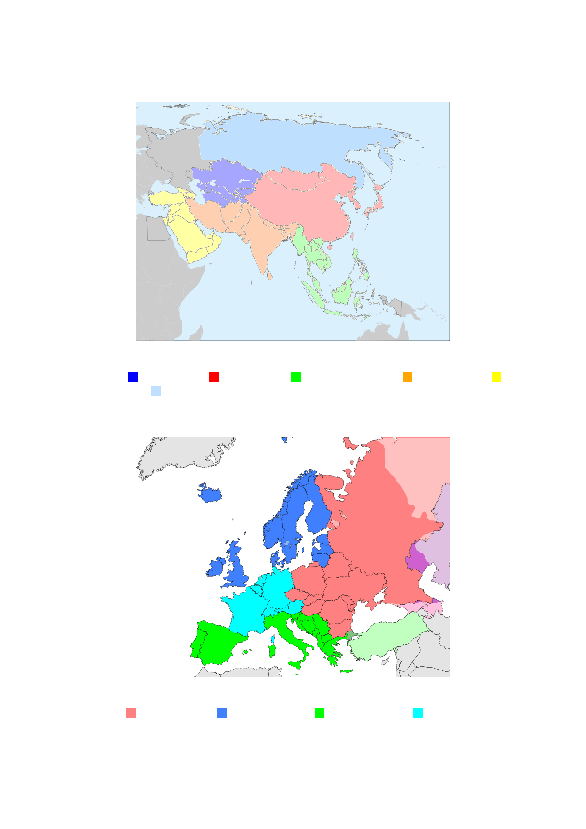
9.2 Technical data: index.json 123
edge) of each mansion, and great circles are drawn from the celestial poles through these stars. In Stellarium,
the defining stars are marked with a little circle. The mansions are quite different in width.
" lu n a r _ s y s t e m " : {
" name ": { " native " : " ... ", " p ronounce ": "Xiù", " engli s h ": " Lunar M a nsion " } ,
" contex t " : " chin e se lunar man s ion " ,
" de f i n i n g_stars ": [ 6 54 7 4 , 6 94 2 7, ... ],
" coordsys " : " equatorial ",
" exten t ": 9 0 ,
" names ": [ { " sym bol ": "1 " , " nat ive ": " ... " , " prono u n c e ": "Jiˇao" , " en g lish ":
↪ " Horn "} ,
{ " symbol " : " 2" , " na tive ": " ... ", " pronounc e " : "Kàng" , " en g lish ":
↪ " Neck "} ,
...
where
"name" cultural name as described in 9.2.7.
"context"
(optional, recommended) context data for all English names in lunar mansions (enhancement
of localization support).
"comment"
(optional) commentary for lunar system, it will be used as extra commentary for translators
also.
"defining_stars" List of HIP numbers of the 28 defining stars.
"coordsys" may be "equatorial" or "ecliptical" (default).
"extent" The zone of interest. The Chinese mansions extend from pole to pole.
"names"
Sequence of names. In addition to the elements listed in 9.2.7,
"symbol"
provides a Unicode
symbol or 1-2 letter string (for practical reasons, a number seems generally useful). The number of
entries must be equal to (or larger than) the number of elements of
"defining_stars"
. Excessive
entries are ignored.
9.2.7 Names of Stars, Planets and Nonstellar Objects
Many cultures have defined their own names for stars, planets and even a few deep-sky objects bright enough
to be seen with the unaided eye. The
"common_names"
dict in a skyculture file
index.json
contains entries
of arrays tagged with HIP catalog numbers or other names.
Names for stars, constellations, asterisms, planets and DSOs can be specified with a plethora of options:
v 25.2
"native" name in the original language of the skyculture.
"english" translation of the name’s meaning. This is translated to users’ language.
"pronounce"
(optional, but recommended) a Latin-character based transliteration/pronunciation aid, re-
quired when
"native"
is written in non-Latin-based glyphs (e.g., Chinese, Arab, Hindu, Tibetan,
. . . ), e.g. Pinyin for Chinese. This is usually written with simple characters found on typewriters and
may also be translated to user language to adopt different customs.
"transliteration"
(optional) a scientific Latin-character based transliteration where applicable. Not
translatable to user language, but may use extended diacritics. The scheme may not be helpful as
pronunciation aid. For example, Wylie for Tibetan.
"IPA" (optional) International Phonetic Alphabet, a standardardized phonetic spelling.
"byname"
an optional explanatory addition to the name for constellations and stars only. May be helpful
v 25.3
to explain mythological figures. This is translated to users’ language, but is not included in search
functions.
"context"
(optional) Short english explanation that helps to disambiguate terminology. Not displayed in
the program.
"translators_comments" (optional): comments to be shown to translators on Transifex.
"references" (optional): array of integers, referring to the references list in description.md.
As example, we show a part of the Samoan skyculture:
" co m m o n _ n a m e s " : {
" HIP 32349 ": [ { " englis h " : " Glid i ng Star ", " nati ve ": "F¯et¯usolonu
‘
u"}] ,
" HIP 68702 ": [ { " englis h " : " Mea " , " nati ve ": " Mea "}] ,
" HIP 71683 ": [ { " englis h " : " Filo ", " nati ve ": " Filo "}] ,
" M45 ": [ {" engl ish ": " Face of Li
‘
i", " native ": "Mat¯ali
‘
i"}] ,
" NGC205 5 " : [ {" eng lish ": " Pale Cl oud ", " nati ve ": " Aotea " } ] ,
" NGC29 2 ": [ { " englis h ": " Fly ing Cloud ", " nati ve ": " Aolele " } ] ,
" NGC609 3 " : [ {" eng lish ": " Pae "} ],
" NGC612 1 " : [ {" eng lish ": " Suga "}] ,
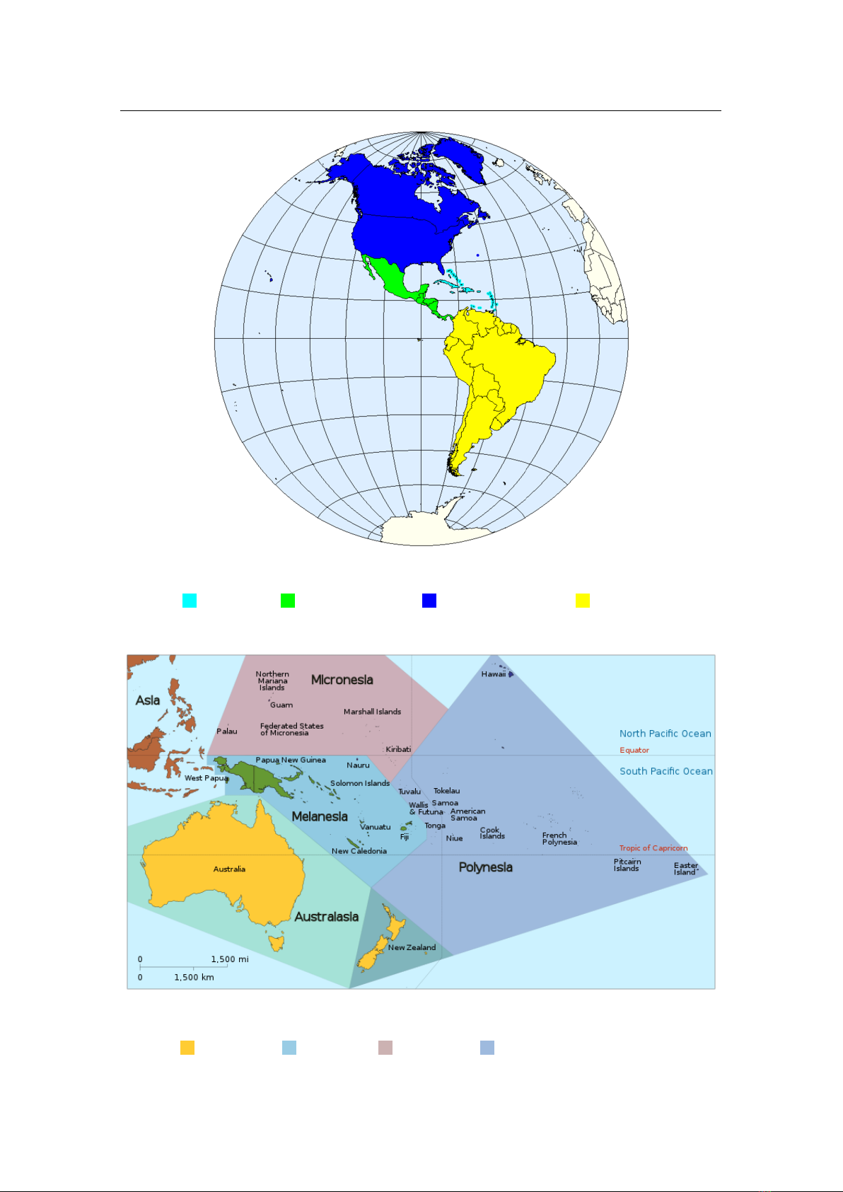
124 Chapter 9. Sky Cultures
" NAME Earth " : [ {" eng l ish ": " Eart h " , " na tive ": " Lalolag i " } ] ,
" NAME Jup iter ": [{ " engl ish ": " Un dying Mys tery " , " native ": "Tupual¯egase"} ] ,
" NAME Mars ": [ { " englis h " : " Redd i sh Face / S urface " , " na tive ": " Matamemea " } ],
" NAME Mer cury ": [{ " engl ish ": " Br o w nish " , " native " : " Ta ' elo " }] ,
" NAME Moon ": [ { " englis h " : " Moon ", " nati ve ": "M¯asina"} ],
" NAME Sa turn ": [{" en glish ": " Garla n d Star ", " nativ e ": "F¯et¯u
‘
¯asoa"} ],
" NAME Sun ": [ { " engli sh ": " Sun " , " na tive " : "L¯a"} ] ,
" NAME Venus " : [ {" eng l ish ": " Mo rning Star / F o r bidden Radia n ce " , " nativ e ":
↪ " Tapu ' itea "} ]
}
9.2.7.1 No translation in Modern Skyculture?
The star names that have been collected over the years in our default Modern skyculture come from an
extensive collection of sources. Some names from Latin and Arab sources have a well-known meaning. In
contrast to what we recommend for non-modern skycultures, we still keep the original name as translation in
the
"english"
string, as such names are used internationally, without thinking about the translated meaning.
Translated names may show slight, language dependent, spelling variations, or transliterations to other glyph
systems, though. At best, the "byname" can transport a translation of the meaning to user language.
9.2.7.2 Star names
The Keys for stars generally start with
"HIP "
. The associated array contains again dicts providing
"native"
(original) and
"english"
(translatable) spellings of the star names, and
"references"
(optional but highly
recommended) which indicates in which sources (see 9.1.2) these star names or particular spellings occur.
The
"english"
name will be translated. An additional
"native"
entry can be given, which is the culture-
native version of the spelling (also in language-specific glyphs when available in UTF8 and the current font)
and will never be translated but can be shown on screen if so configured.
" c o mmo n_n ame s ": {
" HIP 6 7 7 " : [{ " nat i ve " : " Alpher atz " , " eng l ish " : " Al phe r atz " , " re f er e nce s ": [1
↪ , 2 , 5 ,6 ,1 1 ,12 ,3 7] } ,
{" n ative " : " Si r rah " , "e n glis h ": " Sirr a h " , " r e fer e nce s " : [ 23 ,3 7] }] ,
" HIP 7 4 6 " : [{ " nat i ve " : " C aph " , " en g lish " : " Caph " , " r efe ren c es " : [1
↪ , 2 , 6 ,1 1 ,12 ,2 3 ,37 ]} ,
{" n ative " : " Al S a nam al Nakah " , " en g lish ": "Al Sanam al Nakah " , " re f ere n ce s ": [37 ]} ] ,
... }
When there is more than one name for a star, the first in the list is used as screen label.
9.2.7.3 Planet Names
The "common_names" array can also contain dicts of native names of the planets. For these, the JSON key
is formed from
"NAME "
, a space and the English name of the planet. The value array provides the dict
entries ("native", "english", . . . ) listed above.
Currently, if more than one
"english"
strings are given, the first is used as screen label. This may
change as the features further evolve.
In some cultures, Venus and even Mercury may have different names, depending on evening or morning
v 25.2
visibility. We can add a tag
"visible"
which may be either
"morning"
or
"evening"
to select the name.
If the base name should be the screen label, you must repeat it as first entry of the object’s
"NAME "
name
array. If the elongation-dependent name should be screen label, place the names with
"visible"
first, then
repeat the standard name to be shown in the Info text. See the examples for Venus as Morning Star and
Evening Star in the modern skyculture.
In earlier versions it was recommended to combine the native name with an English translation. In the
new format here we should keep them separate, and the actual screen label can be combined from available
components on the fly (see 4.4.6).v 25.2
9.2.8 Deep-Sky Objects Names
"common_names"
can also contain native names for deep-sky objects (DSO). The content of the dicts is
similar to the format for planet names above. Known tags are
"english" English meaning
"native" (optional) Native name. May be in native glyphs when supported in UTF8.
"pronounce" (optional) Native name in European glyphs, if needed. For Chinese, expect Pinyin here.
"transliteration"
(optional) Scientific transliteration of the native name in European glyphs, if needed.
"IPA" (optional) International Phonetic Alphabet.
"context"
(optional) Short english explanation that helps to disambiguate terminology. Not displayed in
the program.

9.2 Technical data: index.json 125
"translators_comments"
(optional) English explanations that help in translation. Not displayed in the
program.
"references" (optional) the sources for these names where applicable
9.2.9 User Settings for the Skycultures
The large number of label combinations requires storing them in a user accessible way. In essence, we are
v 25.2
using a 6-bit scheme with name elements that either show up or are omitted.
Native to show the native name in native glyphs.
Pronounce to show a Latin-character based transliteration usable as pronunciation aid.
Translit to show a scientific transliteration that is not necessarily aimed at pronunciation.
Translated to show the meaning of the name translated to user language.
IPA to show the name in International Phonetic Alphabet.
Modern to show the contemporary scientific object name.
The names for the active parts are joined with commas (the sequence of entries is irrelevant and does not
influence displayed order), and the resulting strings stored in config.ini in two dedicated sections like:
[ SC InfoLabe l S t y l e ]
arabic _ a r a bia n _ p e nins u l a = Native , P ronounce , Mode rn
bo o rong = Native , Translate d
ch i nese = Native , Pronounce , Translated , Mod ern
mo dern = Native , Mod ern
russian_siber i a n = Native , Pronounce , Translit , Translat ed , IPA , Modern
[ SCScreenLabe l S t y l e ]
arabic _ a r a bia n _ p e nins u l a = Pronounce , Translated , Moder n
aztec = Native , Translated
ch i nese = Pronounce , Transla ted , Mod ern
mo dern = Native , Mod ern
russian_siber i a n = Pronounce , Transla ted , Mod ern
9.2.9.1 Not enough, or too many names?
Over the years, we have collected a quite extensive list of star names from many references. Until recently,
the scientific community was not interested in standardizing names. With the introduction of Exoplanet
naming contests, the International Astronomical Union started to also be concerned with the names of the
brighter stars, and a proper Working Group on Star Names has formed.
Stellarium comes with a list of standardized names in
skycultures/common_star_names.fab
. These
are always used when a skyculture shows
"fallback_to_international_names"
(see 9.2). If you always
want to see these names, regardless of whether they are used or not in the respective skyculture, add the
following to your config.ini:
[ viewing ]
fl ag _s ky cu lt ur e_ al wa ys _fallback_to_internatio na l_ na me s = true
Activating this flag for non-modern skycultures may feel weird, though, as it mixes these names into the
other-cultural namespace.
Excluding excessive names
In contrast, some of the collected names may be too fanciful for your taste. If you can identify that those
v 25.2
names that irritate you all come from a single or just a few entries of the reference list, you can exclude those
sources, and thus the names they bring into the program. Note that if a fancy name comes from more than
one book, you would have to exclude all books to ban that name from your display.
In a similar way, some of the collected asterisms (secondary figures), especially in the default Modern sky
culture, may be too much for you. There are overlapping entries like the “Winter Hexagon” vs. “Heavenly
G”, or parts of constellations like Orion’s shield and cudgel are marked as asterism. Some users may find
that this clutters their screens too much. If you cannot identify a reference which introduces the unwanted
asterism (for some entries we cannot specify a source, unfortunately), you can also exclude them by their
unique abbreviation, which is the last part of their "id" entries.
To exclude entries from being displayed for a particular skyculture, add an entry like this to
config.ini
:
[ S CExclud eRefere nces ]
modern = 11 ,36 , OrB , OrS , OSh ,OrC ,HeG ,Sal , TPT

126 Chapter 9. Sky Cultures
Here,
modern
names the skyculture, and the comma-separated entries are references listed in the file
description.md or asterism abbreviations you want to be ignored.
9.3 Terr itory description
Most traditional skycultures are regional. The map interface in the View dialog should indicate where on
v 26.1
Earth a skyculture is located. Stellarium makes use of a file in the GeoJSON format,
territory.geojson
,
to encode where and when this culture is located. In case a cultural group can be traced over a longer time
and the culture has moved or spread, the time slider below the map will show the changes in the geographic
regions.
GeoJSON is a flexible and simple JSON-based format to encode a collection of geographic features
(points, lines and polygons) with geographic coordinates (pairs of longitude/latitude in decimal degrees,
WGS84). Additional properties can be given in a
"properties"
dictionary. Stellarium only uses polygonal
features, and stores
"beginDate"
and
"endDate"
data (calendar years) for each polygon. If the end date
should be “now”, this is indicated by a special value 9146.
An example (Norse (Edda) SC):
{
" type ": " FeatureCollec t i o n " ,
" features " : [
{
" type ": " Feature " ,
" pr o p erties ": {
" be ginTime ": 80 0 ,
" endTim e " : 1 40 0
} ,
" geometry " : {
" co o r d i n a tes ": [
[
[ -2 2 . 74 6 44 2 92 1 5 26 3 24 , 6 4 .1 3 2 94 9 59 3 28 3 9 7 ] ,
[ -2 2 . 43 7 76 2 17 9 2 97 2 45 , 6 4 .0 3 1 76 5 02 1 70 1 2 9 ] ,
...
[ -2 2 . 81 8 12 7 60 2 7 43 7 8, 64.0 8 8 85 2 23 3 0 67 7 7 ]
]
] ,
" type ": " Polygon "
}
} ,
...
]
}
9.4 The Skyculture Converter
Many sky cultures have been created and maintained outside of Stellarium. They follow the old format,
which is no longer supported since Stellarium version 25.1. To ease the transition we have developed a
converter tool. It is a console application that takes a path to the old-format sky culture directory, and a path
where to put the converted sky culture.
The converter is installed together with the program, but there is no menu entry for it. On Windows,
press the Windows key and type cmd to startup the command console.
Let us assume you have created a skyculture following the format used until version 24.4 and described
in previous editions of this Guide, and that this skyculture
mine
resides in the default user data directory on
Windows (see 5.1 for other platforms). First we rename the skyculture to indicate that it is old and outdated.
Then we must call the converter in its absolute path name, with names of old (source) and new (target)
directories as program arguments.
Example command to run it:
cd c :\ Users \< ME >\ AppDa ta \ Roam ing \ s kyc ul tur es
move mine mine . old
"c :\ Program Files \ s tel lar ium \ skyculture - conve rte r " mine . old mine
While the converter tries hard to convert the description text from HTML to Markdown adding some
sections from other parts of the sky culture, the conversion result may not be perfect. Formerly the description

9.5 Publish Your Work 127
was completely free in structure, while now there are some structural requirements on it, so the text may
need some editing to conform.
If you have gettext translation files (the ones whose names are in the form
locale-name.po
) for the
names of stars, constellations etc., you can pass the path to the directory that contains them as an optional
third positional argument to the converter.
Additionally, there are some options that you can use to control the conversion:
--footnotes-to-references
Convert footnotes in a particular form to references. Such footnotes are
expected to be in the form of
<p id =" footnote -9 " > This is a foo tnote </p>
while the references to them are expected to be in the form of
<sup ><a href = "# footnote -9 " > [9] </ a></ sup >
--untrans-names-are-native
Put the names that in
star_names.fab
or in
dso_names.fab
are de-
noted without an underscore into the
"native"
section of the name, rather than
"english"
. For
example, with this option
32349|("F¯et¯usolonu
‘
u")
would be used for the
"native"
name, while
32349|_("Gliding Star") would be used for the "english" tag.
--native-locale LOCALE
In addition to files
star_names.fab
or
dso_names.fab
, some sky cultures
have localized versions of them, like e.g.
star_names.zh_CN.fab
, that were never actually used
but do contain useful information. If you pass the locale (
zh_CN
in this example) as the
LOCALE
parameter, these names will be read and put into the
"native"
section of the corresponding JSON
entry. Note that the order of stars/DSOs in the normal and localized files must be the same, otherwise
there’s no way to match the names.
--translated-md
To check the look of the translated description texts you can use this option. The output
directory will contain files named like
description.es_419.DO_NOT_COMMIT.md
, in addition to
description.md
, with the
DO_NOT_COMMIT
part reminding you that they are not a part of the sky
culture.
After the run, read the notes and warnings, and adjust your text accordingly. Make especially sure to prepare
and adjust your old
description.en.utf8
for successful conversion. For example, it must start with an
HTML header of level
<h1>
(the only such header in this file!) which is expected to match the skyculture
name given in the old info.ini. If in doubt, the latter will be used in the new files.
Generally, clean HTML should be converted successfully. Given the wide variety of writing styles, not
every conversion may however work flawlessly, and you may have to adjust the result, also in light of the
new features. To protect any changes you may have added after conversion, running the converter again
needs a new target directory.
9.5 Publish Your Work
If you are willing to let other users enjoy the result of your hard work (and we certainly hope you do!),
when you are done, please write a note in the Forum or at GitHub. We will decide about acceptability and
classification, or may ask for better descriptions for the benefit of our users.
Please put the imagery and text under some compatible open-source license (see 9.1.3). Else the sky
culture cannot be hosted by us. While we cannot be held responsible for legal problems, it seems that CC BY
4.0 International
6
or CC BY-SA 4.0 International
7
licenses are best suited. See notes in section 9.1.3 above.
6
https://creativecommons.org/licenses/by/4.0/
7
https://creativecommons.org/licenses/by-sa/4.0/

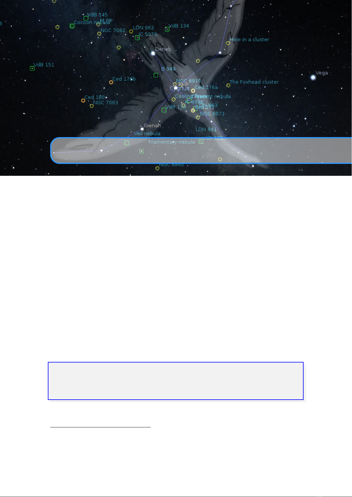
10. Surveys
GUILLAUME CHÉREAU
10.1 Introduction
A sky survey is a map of the sky stored as a hierarchical set of a potentially large number of smaller images
(called tiles). The advantage compared to a regular texture is that we need to render only the visible tiles of
a potentially gigantic image at the lowest resolution needed. This is particularly interesting for rendering
online images that can be stored on a server, while the client only has to download the parts he currently uses.
Since version 0.18.0, Stellarium added some preliminary support for loading and rendering online
surveys in the Hierarchical Progressive Surveys (HiPS) format, developed by the International Virtual
Observatory Alliance. A full description of the format can be found on the IVOA website
1
.
10.2 Hipslist file and default surveys
Hipslist files are text files used to describe catalogs of HiPS surveys. The full specification is part of the
HiPS format, and looks like that:
# Exa m ple of a h i pslist file .
# Date : 2018 -03 -19
obs _ t i tle = call i s to
hips_service_ u r l = https :// data . stellarium . org / survey s / cal l i sto
hips_relea s e _ d a t e = 2018 -03 -18 T14 :01 Z
hips_s t a t u s = pub lic mi rror clonableOnce
...
Stellarium by default tries to load HiPS from two sources:
•
http://alasky.u-strasbg.fr/MocServer/query?*/P/*&get=record (deep sky)
•
https://data.stellarium.org/surveys/hipslist (planets)
This can be changed with the
sources
entries in the
[hips]
section of the configuration file (see also
section D.1.30). You can add your own private HiPS surveys by either running your own (even machine-local)
webserver, or just placing your files into any directory and adding a file:// URL:
[ hips ]
so u rces /1/ url = http :// ala sky .u - s t rasbg .fr / M o c S erver / query ?*/ P /*& get = reco rd
so u rces /2/ url = ht tps :// data . stellariu m . org / survey s / hip s list
so u rces /3/ url = http :// localhos t / Stella r i u m / hips / hipslist
so u rces /4/ url = file :/// D:/ S t ellarium / h ips / hi pslist
so u rces / size = 4
1
https://www.ivoa.net/documents/HiPS/20170519/REC-HIPS-1.0-20170519.pdf

130 Chapter 10. Surveys
10.2.1 Finetuning HiPS surveys
Sometimes it is useful to alter the rendering of sky HiPS surveys. The layer appearance controls allow
v 26.3
users to adjust gamma, saturation, contrast, brightness, opacity, and the displayed color channel for each sky
survey layer. Opacity is especially useful when displaying more than one survey at the same time, or when
combining monochrome surveys in different color channels.
Users can also invert the colors of a layer, which can be helpful for surveys or historical sky maps
with a bright background. Optionally, atmospheric extinction can be applied to sky HiPS layers, making
optical color surveys appear more photo-like when shown together with a foreground landscape. The layer
appearance controls do not apply to planetary HiPS textures.
10.3 Solar system HiPS survey
Though not specified in the HiPS standard, Stellarium recognises HiPS surveys representing planet textures,
as opposed to sky surveys. If the
obs_frame
property of a survey is set to the name of a planet or other solar
system body, Stellarium will render it in place of the default texture used for the body.
10.4 Digitized Sky Survey 2 (TOAST Survey)
GEORG ZOTTI, ALEXANDER WOLF
The older way to provide a tessellated all-sky survey uses the TOAST encoding
2
. Stellarium provides access
to the Digitized Sky Survey 2, a combination of high-resolution scans of red- and blue-sensitive photographic
plates taken in 1983–2006 at Palomar Observatory and the Anglo-Australian Observatory.
3
To enable access to the DSS layer, see section 4.3.3 and enable the DSS button. Then just press that
DSS button in the lower button bar, wait a moment, zoom in and enjoy!
10.4.1 Local Installation
This display normally requires access to the Internet. However, in some situations like frequent and extensive
use in fixed observatories, or use in the field when Internet connection is not possible, you can download all
image tiles to your local harddisk for local use. Please be considerate, don’t waste bandwidth, and do this
only if you really need it.
The images are stored in subdirectories that increase in size and number of files (see Table 10.1).
Zooming in loads the next level if available.
Level No of files Filespace (kB)
Level No of files Filespace (kB) Level No of files Filespace (kB)
0 1 32 4 256 7.172 8 65.536 1.661.808
1 4 124
5 1.024 27.920 9 262.144 6.119.092
2 16 472
6 4.096 109.628 10 1.048.576 20.250.216
3 64 1.820
7 16.384 429.800 11 4.194.305 83.583.724
Table 10.1: Number of files and storage requirements for local DSS TOAST installation
For partial downloads, you can limit the maximally used level (e.g. 9 or 10). The difference from level
10 to 11 is really hardly noticeable, yet level 11 contains almost 75% of all data. On a small system like
Raspberry Pi 3, you may run into troubles with too little texture memory when level is more than 7.
Another issue: the level 11 subdirectory holds over 4 million files. Windows Explorer is not optimized
to open and display this number of files and will take a long time to open. Just unpack this archive, but don’t
access the folder with Explorer.
If all that does not discourage you, you can download the archives at
https://dss.stellarium.org
/offline/.
Then add a few entries to the
[astro]
section in Stellarium’s
config.ini
. On Windows, if you have
a harddisk
T:
with path
T:\StelDSS
that contains the unpacked image subdirectories 0, 1, 2, . . . , 10, the
section may look like
[ astro ]
to as t_sur ve y_direc tory = StelDSS
2
Please see http://montage.ipac.caltech.edu/docs/WWT/ for details
3
The original data are available at https://archive.stsci.edu/cgi-bin/dss_form.

10.4 Digitized Sky Survey 2 (TOAST Survey) 131
to ast_s urvey _host = T :/
to ast_sur vey_l evels = 10
On Linux, with the files stored in
/usr/local/share/Stellarium/StelDSS
, the same section could look
like
[ astro ]
to as t_sur ve y_direc tory = usr / local / share / S tel lar ium / Stel DSS
to ast_s urvey _host = /
to ast_sur vey_l evels = 10

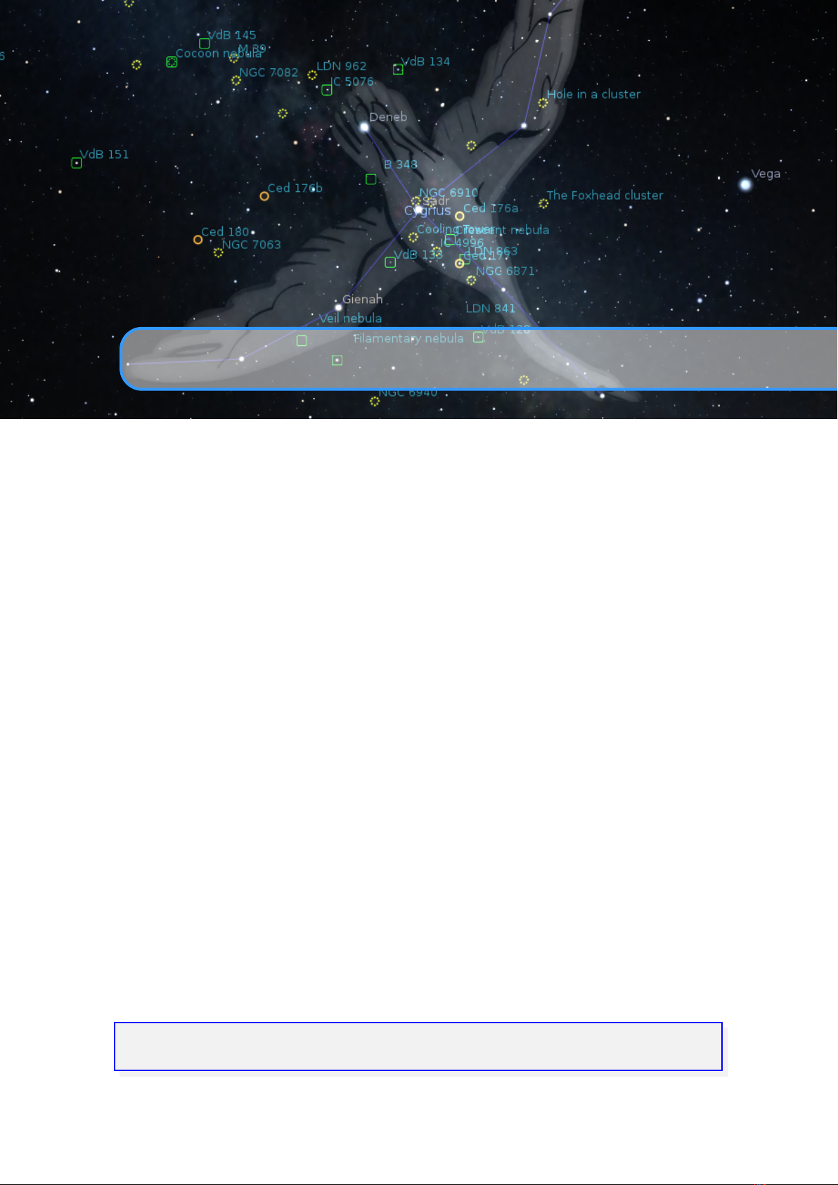
11. Stellarium’s Skylight Models
GEORG ZOTTI
11.1 Introduction
Stellarium’s main aim is a realistic simulation of the night sky. This is more than just the creation of a star
map. Especially a realistic simulation of twilight and the visibility of stars, deep-sky objects or the Zodiacal
light is a challenge. Since early in its history Stellarium has used models from the computer graphics
literature to achieve its goals. For most users, the models seem to work well, but more advanced users may
want to tweak some of the values.
11.2 The Skylight Models
11.2.1 Legacy Mode: The Preetham Skylight Model
A well-known fast computer graphics model for daylight has been presented by Preetham, Shirley, and Smits
(1999). Its brightness distribution is based on an all-weather model for sky luminance distribution by Perez,
Seals, and Michalsky (1993) and models chromaticity distribution with similarly-shaped functions. It works
reasonably well for average conditions, and a “turbidity” parameter
T
allows a simple modelling of visibility
conditions. In terms of the atmospheric extinction coefficient k (see 19.13.1), we can define
T = 25(k − 0.16)+ 1 (11.1)
In Stellarium, a value of
T = 5
has been used for many years, and the chromaticity parameters have been
slightly changed for a more pleasing color distribution at this value for
T
. Recently, we have made the many
parameters of the Preetham model accessible for users to fine-tune. Not many users will even want to do this,
and therefore you must enable this manually by editing config.ini:
[ Skylight ]
enable_gui = true
Only with this setting, a button will be available in the View settings, Sky tab (section 4.4.1.2).
All settings described here will immediately be stored in config.ini.
One setting allows to compute T from k with the above relation 11.1.
Please note that the parameters are far from intuitive, therefore we added two sets of reset functions. One
sets the values to those in the original paper, the other re-establishes Stellarium’s sky colors from version
0.21.3 and earlier, which however seem only suitable for T = 5.

134 Chapter 11. Stellarium’s Skylight Models
A sky brightness model better suited for astronomical simulation, including twilight and brightness
contributions of the Moon and airglow, was presented by B. E. Schaefer (1989-93 and 1993). By default,
Stellarium uses this model in combination with chromaticity from the Preetham model. For experiments,
you can however revert from the Schaefer brightness model to the Preetham model. The parameters of the
Schaefer model are currently not accessible for further experiments.
Some more parameters fine-tune some aspects of rendering of the Solar disk and the solar glare. It makes
a slight difference whether the Sun’s disk is plotted before or after the glare, and whether the solar sphere is
rendered after the atmosphere.
11.2.2 Advanced Mode: The ShowMySky Skylight Model
A much more advanced skylight model has been presented by Bruneton and Neyret (2008). An implementa-
tion of this has been developed by Ruslan Kabatsayev just in time for inclusion in version 1.0. Switching
between the models is described in section 4.4.1.2.
It requires graphics hardware which uses OpenGL 3.3 or better and consists of two components.
Atmospheric data (a description of gas composition) is processed by an auxiliary program, CalcMySky,
which creates a lot of textures and shaders. For final display, a software component (the ShowMySky library)
is used that processes these data in real-time to compute the final sky colors. This model and its default
atmosphere data especially can deliver stunning reality of twilight colors in a dry atmosphere, and also
provides special modes for the “circular twilight” during a Total Solar Eclipse.
To choose a dataset
press near the Path to data entry field, and in the dialog that opens, choose the
directory with the dataset. Stellarium comes with a default dataset that’s automatically chosen after a
fresh installation. Power users can use CalcMySky
1
to generate other atmospheres. Creating a new
dataset requires some understanding of the physics of light scattering.
Eclipse simulation quality
option lets you configure the balance between realism of skylight simulation
during a solar eclipse. The values of this option can be:
0
This is the fastest and crudest mode. The atmosphere is simply dimmed to account for the lower
amount of direct sunlight.
1
This is the first mode that actually tries to simulate an eclipse. It uses precomputed textures, and
may look blocky in some cases like e.g. very low Sun (and Moon).
2
This mode is much slower than the previous one (2.5 FPS on an NVIDIA GeForce GTX 750Ti).
In this mode part of the calculation is done on the fly for the current eclipse phase to improve
correctness of the simulation, unlike the previous mode where a texture was used that contains
data only for totality, other phases being approximated from this.
3
This is the slowest mode (1.1 FPS on NVIDIA GeForce GTX 750Ti), but computation is done on
the fly for the whole simulation, which yields best quality.
To achieve higher frame rates on slow systems, the configuration parameter in config.ini:
[ landscape ]
at mo sp here_reso lu ti on_reduct io n = 4
allows reducing the resolution of the skylight texture. Preferred values are:
1 full resolution (default)
2 half resolution
4 quarter resolution
The configuration switch in config.ini:
[ landscape ]
fl ag _a tm osphere_d yn am ic_resoluti on = true
allows to use the reduced resolution only while moving the view, when panning, zooming, dimming
or in time-lapse mode. With the real-time display, on the other hand, the full resolution is retained.
Possible values are:
false static resolution (default)
true dynamic resolution
1
https://github.com/10110111/CalcMySky

11.3 Light Pollution 135
Note:
In dynamic resolution mode, a motion analyzer selects either full or reduced resolution. The change
in resolution could be particularly visible in close proximity to the Sun. Especially at full resolution,
frames will be skipped depending on the speed of movement.
A more detailed description of how to create a custom atmosphere will be given in a future version of this
User Guide.
11.2.3 Intermediate Mode: The Lightweight Skylight Model
This model combines a realistic view of the sky as in ShowMySky with light weight of the Preetham model,
v 26.2
at the cost of being fixed to simulating a sea level sky (just as Preetham), lacking the realism of eclipse
simulation (also as Preetham), and having no parameters to tweak.
The Lightweight model is based on a set of meshes generated from a render of ShowMySky, so its look
is just as realistic (at sea level and without any eclipse) as that of ShowMySky, except for the solar aureole,
which is a bit simplified.
This is the default skylight model that supports the same set of computers as the Preetham model. But
v 26.3
if you use a weak laptop on batteries in the field, you may want to switch to Preetham, which is a bit less
energy consuming.
11.3 Light Pollution
In urban and suburban areas the night sky is lit by ground sources of light. This light is scattered by the
atmosphere, and the sky appears brighter. This reduces visibility of astronomical objects.
Stellarium simulates this effect. The main physical quantity that describes light pollution is zenith
luminance, measured in candelas per square meter (
cdm
2
). It can be measured using a device called sky
quality meter (SQM).
For astronomical observations often another unit of sky brightness is useful: magnitudes per square
arcsecond (magarcsec
2
). It is related to cdm
2
as
L = 10.8× 10
4−0.4M
, (11.2)
where
L
is the value in
cdm
2
, and
M
is the value in
magarcsec
2
. Some SQMs give readings in
magarcsec
2
.
Stellarium supports input in both units.
Another way to characterize light pollution is by defining the naked-eye limiting magnitude (NELM).
Unlike luminance, which, although based on human vision, is well-standardized (in particular, the candela is
part of the SI), NELM is subjective and variable: it is based on human vision, depends on weather conditions,
and is not standardized. In Stellarium the calculations follow B. E. Schaefer (1990). In particular, equation
(18)
is used, assuming observer’s acuity
F
s
= 1
(as suggested in the text as “typical observer”), and absorption
term k
v
= 0.3 (as suggested for “typical weather”).
A related subjective characterization of light pollution is the Bortle Dark Sky Scale, which assigns an
integral number from 1 to 9 to the sky based on its brightness. This scale is described in detail in Appendix B.
Stellarium calculates both Bortle class and NELM for user convenience. They aren’t used in the actual
calculations for visualization.
11.4 Tone Mapping
Tone mapping is the process which attempts to compress the brightness values found in nature into the
range of brightness values which can be achieved on a display device so that an image of a natural scene
looks reasonably natural and realistic. The process has been described by Tumblin and Rushmeier (1993),
Larson, Rushmeier, and Piatko (1997) and Devlin et al. (2002). For low-light conditions like night and the
transitional phase, twilight, special considerations have to be taken, first described by Jensen et al. (2000).
Stellarium’s transformation from skylight model to display colors is based on these papers.
Parameters to tweak the tone mapping can be reached in the view settings dialog after pressing
.
Display max luminance
maximal brightness of the used screen. This used to be
100cdm
2
applicable
for CRT monitors, but more modern screens can achieve much higher luminances of
250cdm
2
or
more, to be found in the spec sheets. Adjust this value to influence the displayed brightness along the
horizon.
Display adaptation luminance
describes the view environment where the screen is set up. For an average
office environment,
50cdm
2
seems a usable default. In an outdoor setting, much higher values are
possible.

136 Chapter 11. Stellarium’s Skylight Models
Display Gamma
describes the exponent of a nonlinear correlation between input values and output lumi-
nance of the screen. Higher values push the average image brightness.
Use extra Gamma term The original implementation of tone mapping included a gamma term which did
not exactly follow the description from Larson, Rushmeier, and Piatko (1997), but looks better (more
colorful) than the implementation without the gamma term. You can now play with it to find your
preferred setting. This flag is only used with the Preetham skylight model.
Use sRGB
The final step of color creation is a transformation from CIE Yxy to some display RGB color
space. Nowadays most monitors can display the sRGB color space, therefore this flag is usually
enabled. Disabling this flag will lead to using the Adobe RGB (1998) color space. The colors may
look a bit better on monitors which are set to display Adobe RGB, but washed-out on sRGB monitors.

III
Extending Stellarium
12 Plugins: An Introduction . . . . . . . . . . . . . 139
12.1 Enabling plugins . . . . . . . . . . . . . . . . . . . . . . . . 139
12.2 Data for plugins . . . . . . . . . . . . . . . . . . . . . . . . 139
13 Interface Extensions . . . . . . . . . . . . . . . . 141
13.1 Angle Measure Plugin . . . . . . . . . . . . . . . . . . . 141
13.2 Equation of Time Plugin . . . . . . . . . . . . . . . . . . 143
13.3 Pointer Coordinates Plugin . . . . . . . . . . . . . . . 144
13.4 Time Navigator Plugin . . . . . . . . . . . . . . . . . . . 145
13.5 Object Visibility Plugin . . . . . . . . . . . . . . . . . . . 146
13.6 Text User Interface Plugin . . . . . . . . . . . . . . . . . 149
13.7 Remote Control Plugin . . . . . . . . . . . . . . . . . . . 152
13.8 Remote Sync Plugin . . . . . . . . . . . . . . . . . . . . . 155
13.9 OnlineQueries Plugin . . . . . . . . . . . . . . . . . . . . 158
13.10 Sky Culture Maker Plugin . . . . . . . . . . . . . . . . . 159
13.11 Solar System Editor Plugin . . . . . . . . . . . . . . . . 166
13.12 Nebula Textures Plugin . . . . . . . . . . . . . . . . . . . 169
13.13 Calendars Plugin . . . . . . . . . . . . . . . . . . . . . . . 171
14 Object Catalog Plugins . . . . . . . . . . . . . 177
14.1 Bright Novae Plugin . . . . . . . . . . . . . . . . . . . . . 177
14.2 Historical Supernovae Plugin . . . . . . . . . . . . . . 179
14.3 Exoplanets Plugin . . . . . . . . . . . . . . . . . . . . . . . 182
14.4 Pulsars Plugin . . . . . . . . . . . . . . . . . . . . . . . . . . 194
14.5 Quasars Plugin . . . . . . . . . . . . . . . . . . . . . . . . . 196
14.6 Meteor Showers Plugin . . . . . . . . . . . . . . . . . . . 197
14.7 Navigational Stars Plugin . . . . . . . . . . . . . . . . . 200
14.8 Satellites Plugin . . . . . . . . . . . . . . . . . . . . . . . . 203
14.9 ArchaeoLines Plugin . . . . . . . . . . . . . . . . . . . . 208
15 Scenery3d – 3D Landscapes . . . . . . . . 213
15.1 Introduction . . . . . . . . . . . . . . . . . . . . . . . . . . . 213
15.2 Usage . . . . . . . . . . . . . . . . . . . . . . . . . . . . . . . . 213
15.3 Hardware Requirements & Performance . . . . . 214
15.4 Model Configuration . . . . . . . . . . . . . . . . . . . . 214
15.5 Predefined views . . . . . . . . . . . . . . . . . . . . . . . 221
15.6 Example . . . . . . . . . . . . . . . . . . . . . . . . . . . . . . 221
15.7 Limitations . . . . . . . . . . . . . . . . . . . . . . . . . . . . 222
16 Stellarium at the Telescope . . . . . . . . . 225
16.1 Oculars Plugin . . . . . . . . . . . . . . . . . . . . . . . . . 225
16.2 TelescopeControl Plugin . . . . . . . . . . . . . . . . . 238
16.3 Observability Plugin . . . . . . . . . . . . . . . . . . . . . 246
16.4 Mosaic Camera Plugin . . . . . . . . . . . . . . . . . . 247
17 Scripting . . . . . . . . . . . . . . . . . . . . . . . . . . . 251
17.1 Introduction . . . . . . . . . . . . . . . . . . . . . . . . . . . 251
17.2 The Script Console . . . . . . . . . . . . . . . . . . . . . . 252
17.3 Includes . . . . . . . . . . . . . . . . . . . . . . . . . . . . . . 252
17.4 Minimal Scripts . . . . . . . . . . . . . . . . . . . . . . . . . 252
17.5
Critical Scripting Differences introduced with ver-
sion 1.0 . . . . . . . . . . . . . . . . . . . . . . . . . . . . . . . 253
17.6 Example: Retrograde motion of Mars . . . . . . . 253
17.7 More Examples . . . . . . . . . . . . . . . . . . . . . . . . 257

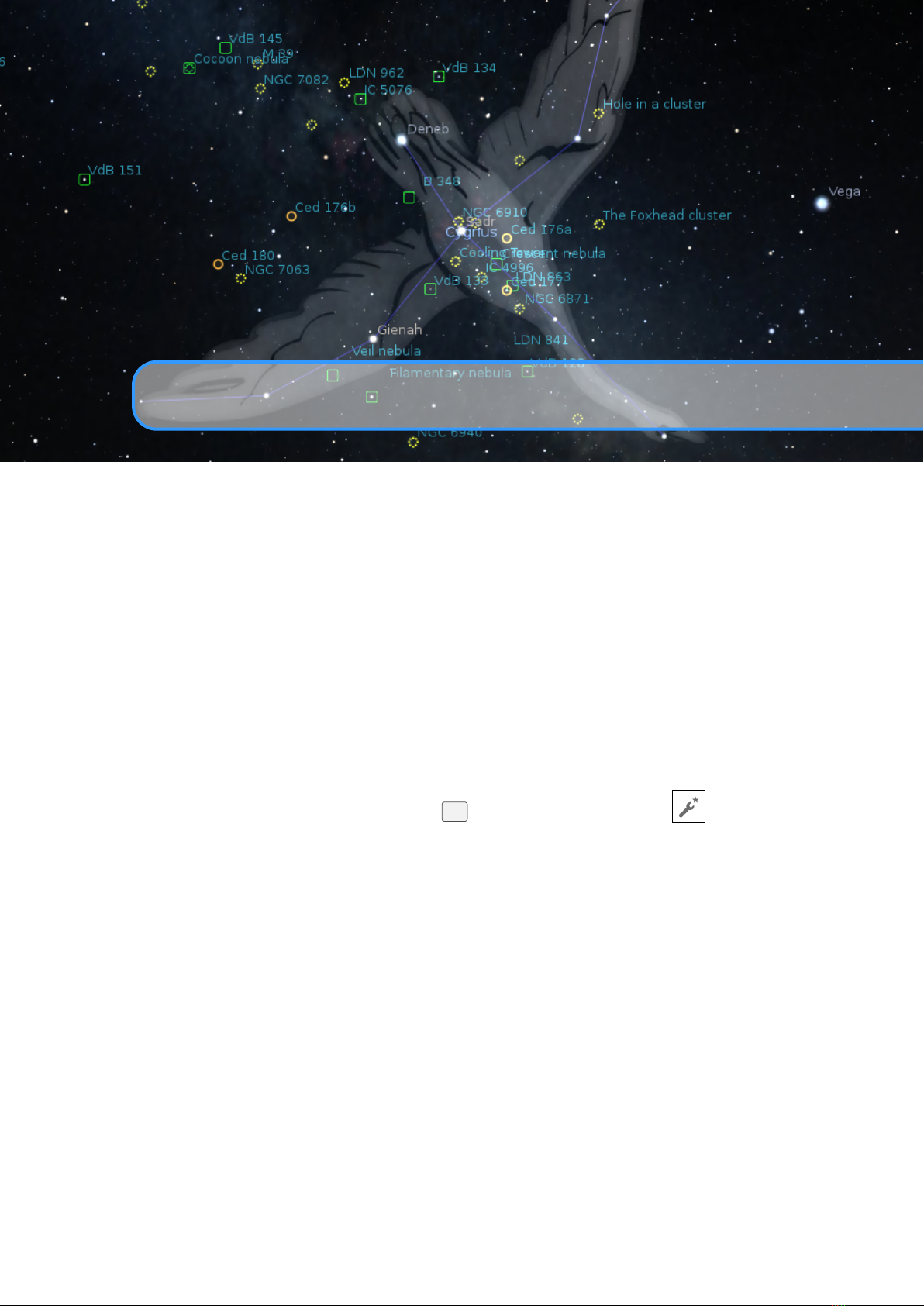
12. Plugins: An Introduction
Starting with version 0.10.3, Stellarium’s packages have included a steadily growing number of optional
extensions called plug-ins which are presented in the following chapters. All these plug-ins are “built-in” in
the standard Stellarium distribution and don’t need to be downloaded separately.
12.1 Enabling plugins
To enable a plugin:
1. Open the Configuration dialog (press
F2
or use the left tool bar button
)
2. Select the Plugins tab
3. Select the plugin you want to enable from the list
4. Check the Load at startup option
5. Restart Stellarium
If the plugin has configuration options, the configuration button will be enabled when the plugin has been
loaded and clicking it will open the plugin’s configuration dialog. When you only just activated loading of a
plugin, you must restart Stellarium to access the plugin’s configuration dialog. The plugin’s configuration
dialog is also available by right-clicking on the respective plugin’s main button in the bottom button bar.
12.2 Data for plugins
Some plugins contain files with different data, e.g., catalogs. JSON is a typical format for those files, and
you can edit its contents manually. Of course, each plugin has a specific format of data for its own catalogs,
and you should read the documentation for the plugin before editing its catalog.
You can read some common instructions for editing catalogs of plugins below. In this example we use
file name catalog.json for identification of the catalog for a typical plugin.
You can modify the
catalog.json
files manually using a text editor. If you are using Windows, it
is strongly recommended to use an advanced text editor such as Notepad++
1
to avoid problems with
end-of-line characters. (It will also color the JSON code and make it easier to read.)
Warning: Before editing your
catalog.json
file, make a backup copy. Leaving out the smallest detail
(such as a comma or forgetting to close a curly bracket) may prevent Stellarium from starting.
As stated in section 5, the path to the directory
2
which contains catalog.json file is something like:
Windows C:\Users\UserName\AppData\Roaming\Stellarium\modules\PluginName
macOS HomeDirectory/Library/Application Support/Stellarium/modules/PluginName
Linux and UNIX-like OS ~/.stellarium/modules/PluginName
1
https://notepad-plus-plus.org/
2
This is a hidden folder, so in order to find it you may need to change your computer’s settings to display hidden
files and folders.

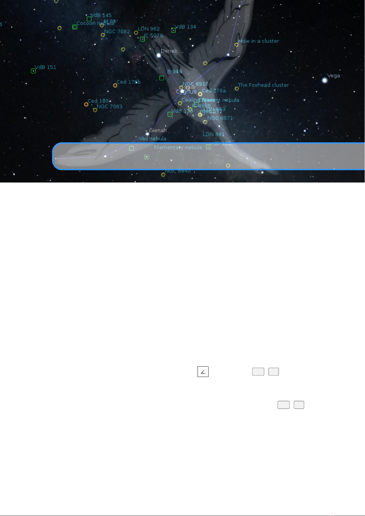
13. Interface Extensions
Most users will soon be familiar with the usual user interface. A few plugins are available which extend the
regular user interface with a few small additions which are presented first. However, some applications and
installations of Stellarium require completely different user interfaces. Mostly, these serve to avoid showing
the user interface panels to an audience, be that in your astronomy club presentations, a domed planetarium
or in a museum installation.
13.1 Angle Measure Plugin
goes misty eyed
I recall measuring the size of the Cassini Division when I was a student. It was not the high
academic glamor one might expect. . . It was cloudy. . . It was rainy. . . The observatory lab had
some old scopes set up at one end, pointing at a photograph of Saturn at the other end of the lab.
We measured. We calculated. We wished we were in Hawaii. A picture is worth a thousand
words.
Figure 13.1: Interface of Angle Measure plugin
The Angle Measure plugin is a small tool which is used to measure the angular distance between two points
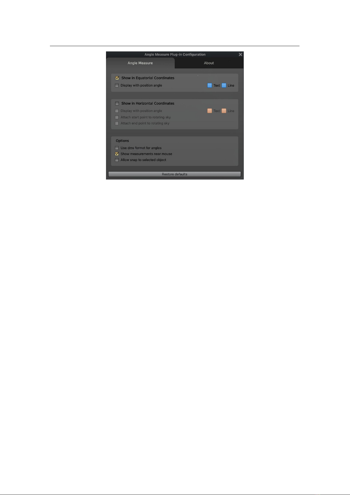
142 Chapter 13. Interface Extensions
on the sky.
1.
Enable the tool by clicking the tool-bar button , or by pressing
Ctrl
+
A
. A message will appear
at the bottom of the screen to tell you that the tool is active.
2. Drag a line from the first point to the second point using the left mouse button.
3. To measure to a different endpoint, click the right mouse button.
4.
To deactivate the angle measure tool, press the tool-bar button again, or press
Ctrl
+
A
on the
keyboard.
In the configuration dialog, you can configure if you want to have distances given on the rotating sphere, or
in horizontal (alt-azimuthal) coordinates. You can also link one point to the resting horizon, the other to the
sky and observe how angles change. You can choose where to display the measurement.
When option “Allow snap to selected object” is activated the process of measurement is changed:
•
The left mouse button is not used for angle measurement, so you can pan the screen and left-click to
select an object as usual.
•
To draw the angle dimension line, you can drag with the right mouse button.
•
A right click moves the end of the angle line that is closest to the mouse pointer.
•
If an object is selected, right-clicking will snap the end of the protractor line (closest to the mouse
pointer) to the selected object.
•
Double-click the right mouse button to capture the end of the line. Another double click with the right
mouse button removes the angle measuring line.
•
Which end of the protractor line is chosen depends on the position of the mouse pointer in relation to
the two ends of the line. The end of the line that is closer to the mouse pointer is moved and defined
as the new end point. The end of the line farther from the mouse pointer is not moved and is defined
as the new starting point.
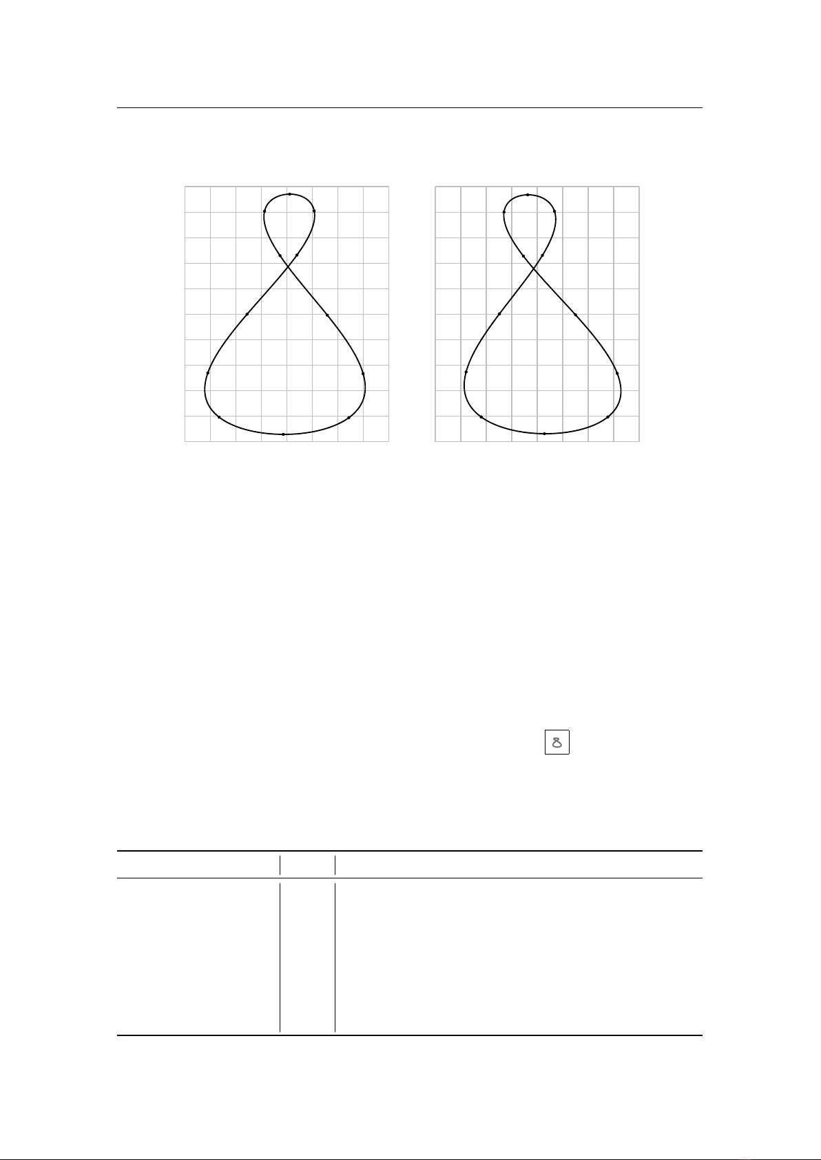
13.2 Equation of Time Plugin 143
13.2 Equation of Time Plugin
-20 -15 -10 -5 0 5 10 15 20
-25
-20
-15
-10
-5
0
5
10
15
20
25
Ari
Tau
Gem
Cnc
Leo
Vir
Lib
Sco
Sgr
Cap
Aqr
Psc
-20 -15 -10 -5 0 5 10 15 20
-25
-20
-15
-10
-5
0
5
10
15
20
25
Ari
Tau
Gem
Cnc
Leo
Vir
Lib
Sco
Sgr
Cap
Aqr
Psc
Figure 13.2: Figure-8 plots for Equation of Time, for years 1000 (left) and 2000 (right). These
plots, often found on sundials, link solar declination (vertical axis) and its deviation at mean noon
from the meridian, in minutes. Labeled dots indicate when the sun entered the respective Zodiacal
sign (30°section of the ecliptic). Figures by Georg Zotti.
The Equation of Time plugin shows the solution of the equation of time. This describes the discrepancy
between two kinds of solar time:
Apparent solar time directly tracks the motion of the sun. Most sundials show this time.
Mean solar time tracks a fictitious “mean” sun with noons 24 hours apart.
There is no universally accepted definition of the sign of the equation of time. Some publications show
it as positive when a sundial is ahead of a clock; others when the clock is ahead of the sundial. In the
English-speaking world, the former usage is the more common, but is not always followed. Anyone who
makes use of a published table or graph should first check its sign usage.
If enabled (see section 12.1), click on the Equation of Time button on the bottom toolbar to display
the value for the equation of time on top of the screen.
13.2.1 Section
[
EquationOfTime
]
in config.ini file
You can edit
config.ini
file by yourself for changes of the settings for the Equation of Time plugin – just
make it carefully!
ID Type Description
enable_at_startup bool Display solution of the equation of time at startup of Stellarium
flag_use_ms_format
bool
Set format for the displayed solution – minutes and seconds or
decimal minutes
flag_use_inverted_value
bool Change sign of the equation of time
flag_show_button
bool Show the tool’s button on the bottom toolbar
text_color
R,G,B Font color for the displayed solution of the equation of time
font_size
int Font size for the displayed solution of the equation of time
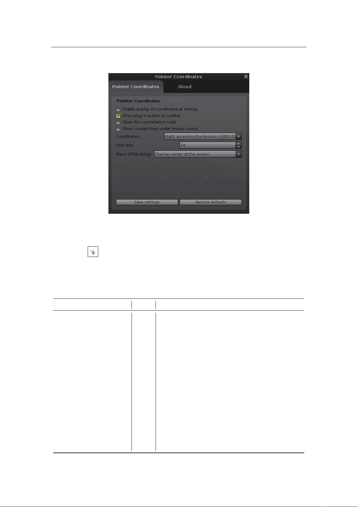
144 Chapter 13. Interface Extensions
13.3 Pointer Coordinates Plugin
Figure 13.3: Interface of Pointer Coordinates plugin
The Pointer Coordinates plugin shows the coordinates of the mouse pointer. If enabled, click on the plugin
button on the bottom toolbar to display the coordinates of the mouse pointer.
13.3.1 Section
[
PointerCoordinates
]
in config.ini file
You can edit
config.ini
file by yourself for changes of the settings for the Pointer Coordinates plugin –
just make it carefully!
ID Type Description
enable_at_startup bool
Enable displaying mouse pointer coordinates at program
startup
flag_show_button
bool Show the plugin’s tool button on the bottom toolbar
text_color
R,G,B Color for coordinates text of the mouse pointer
font_size
int Font size for the displayed mouse pointer coordinates
current_displaying_place
string
Specifies the place of displaying coordinates of the
mouse pointer. Possible values:
TopRight
,
TopCenter
,
RightBottomCorner, Custom. Default value: TopRight.
custom_coordinates
int,int
Specifies the screen coordinates of the custom place for
displaying coordinates of the mouse pointer
current_coordinate_system
string
Specifies the coordinate system. Possible values:
RaDecJ2000
,
RaDec
,
HourAngle
,
Ecliptic
,
AltAzi
,
Galactic. Default value: RaDecJ2000.
flag_show_constellation
bool
Add the 3-letter IAU abbreviation for the constellation of
the mouse pointer location (Roman, 1987).
flag_show_crossed_lines
bool Show crossed lines under mouse cursor.
13.4 Time Navigator Plugin 145
13.4 Time Navigator Plugin
Figure 13.4: Interface of Time Navigator plugin: Time Steps tab (left), Specific Time tab (center),
and Planetary Events (right)
The Time Navigator plugin brings a convenient GUI to many different astronomical time steps and allows
addition or subtraction of one (1) unit of any of these periods interactively. If enabled (see section 12.1),
click on the plugin button on the bottom toolbar to open the plugin window.
The first tab
Time Steps
shows step buttons for different definitions of days, months and years, and even
longer cycles such as the Saros. The second tab
Specific Time
shows buttons to jump to the previous, current
or next event of the selected object, e.g. its meridian transit, as well as buttons for specific twilight moments.
The third tab
Planetary Events
shows step buttons for some interesting planetary events, such as opposi-
tions for outer planets and greatest elongations for inner planets. For the Moon, the four phases (new, first
quarter, full, last quarter) and times for apogee and perigee are shown, as well as times for Earth aphelion
and perihelion. Clicking any of these buttons sets the time to that of the event.

146 Chapter 13. Interface Extensions
13.5 Object Visibility Plugin
The Object Visibility plugin provides map-based tools which help to answer the question where selected
objects can be seen from, and how the solar twilight zones are distributed on Earth or on other supported
Solar System bodies. If enabled (see section 12.1), click on the plugin button
on the bottom toolbar to
open the plugin window.
Figure 13.5: The Visibility tab of the Object Visibility plugin.
The first tab,
Visibility
, works with the currently selected star or deep-sky object. Press
Calculate
to draw
the visibility limits for the selected object on a world map. The solid curve shows where the object just
reaches the horizon, while the dashed curve marks where it reaches the user-defined “good visibility” altitude.
Additional symbols indicate where the object can pass through the zenith and where it becomes circumpolar
in the northern or southern hemisphere.
The map marker follows the observer’s current location. Activate
Set location by map click
to move the
observer by clicking on the map. The
Sync maps
option keeps pan and zoom synchronised between all map
tabs. The place labels can be enabled with a minimum population threshold, and can optionally be restricted
to labels near the plotted lines.
The second tab,
Twilight limits
, is Earth-only. It shows the latitude limits related to the solstices for the
current epoch, including the equator, tropics, polar circles, and the limits at which the Sun’s lowest or highest
altitude is
−6
°,
−12
° or
−18
°. These correspond to the conventional limits for civil, nautical and astronomical
twilight. The calculation follows the obliquity valid for the current simulation date.
The third tab,
Twilight Map
, follows the planetarium time in real time. On Earth it shades the map
according to the apparent solar altitude. The boundary between day and night uses the upper limb of the
Sun with an allowance for atmospheric refraction, while the additional contours mark civil, nautical and
astronomical twilight. The Sun and Moon symbols show the locations where these bodies are in the zenith.
When the observer is located on another supported Solar System body, the
Twilight Map
tab switches
to a simpler terminator view. In this mode the plugin uses the Sun’s centre and the geometric horizon, and
shades the night side of the current body. This is useful for planning observations or surface views from the
Moon, planets, Pluto, or the Galilean satellites supported by Stellarium’s location system.
13.5 Object Visibility Plugin 147
Figure 13.6: The Twilight limits tab of the Object Visibility plugin.
Figure 13.7: The Twilight Map tab on Earth, showing sunrise and sunset, civil, nautical and
astronomical twilight, night, and the subsolar and sublunar points.
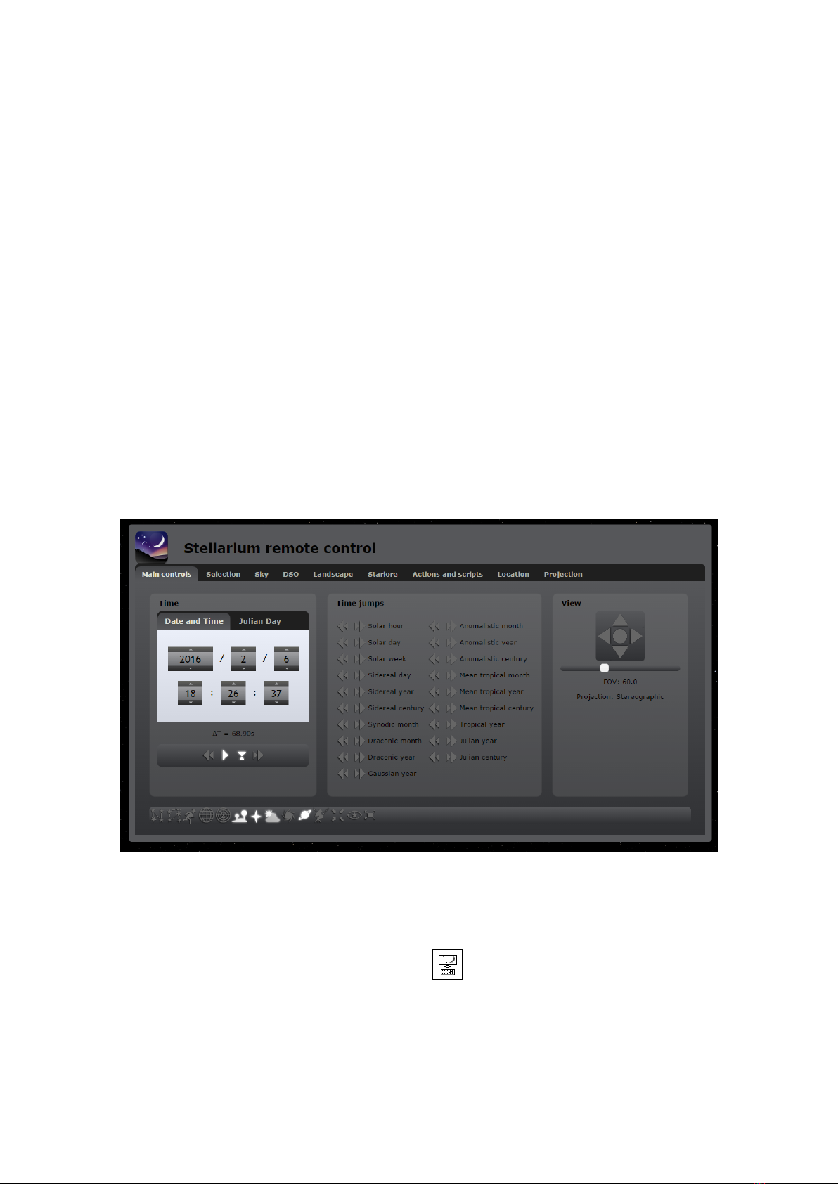
148 Chapter 13. Interface Extensions
Figure 13.8: The Twilight Map tab used from the Moon. On bodies other than Earth, the plugin
shows the geometric solar terminator and shades the night side.

13.6 Text User Interface Plugin 149
13.6 Text User Interface Plugin
This plugin re-implements the “TUI” of the pre-0.10 versions of Stellarium, an unobtrusive menu used
primarily by planetarium system operators to change settings, run scripts and so on.
13.6.1 Using the Text User Interface
1. Activate the text menu using the
Alt
+
T
key.
1
2. Navigate the menu using the cursors keys.
3.
To edit a value, press the right cursor until the value you wish to change it highlighted with > and <
marks, e.g. >3.142<. Then press the cursor keys and to change the value. You may also type
in a new value with the other keys on the keyboard.
13.6.2 TUI Commands
1 Location (menu group)
1.1
Latitude Set the latitude of the observer in degrees
1.2
Longitude Set the longitude of the observer in degrees
1.3
Altitude Set the altitude of the observer in meters
1.4
Solar System Body Select the solar system body on which the observer is
2 Set Time (menu group)
2.1
Current date/time
Set the time and date for which Stellarium will generate the
view
2.2
Set Time Zone (disabled in 0.15)
2.3
Days keys (disabled in 0.15)
2.4
Startup date/time preset
Select the time which Stellarium starts with (if the “Sky Time
At Start-up” setting is “Preset Time”
2.5
Startup date and time
The setting “system” sets Stellarium’s time to the computer
clock when Stellarium runs. The setting “preset” selects a
time set in menu item “2.4 - Startup date/time preset”
2.6
Date Display Format
Change how Stellarium formats date values. “system_default”
takes the format from the computer settings, or it is possible
to select “yyyymmdd”, “ddmmyyyy” or “mmddyyyy” modes
2.7 Time Display Format
Change how Stellarium formats time values. “system_default”
takes the format from the computer settings, or it is possible
to select “24h” or “12h” clock modes
3 General (menu group)
3.1
Sky Culture
Select the sky culture to use (changes constellation lines,
names, artwork)
3.2
Sky Language Change the language used to describe objects in the sky
3.3
App Language Change the application language (used in GUIs)
4 Stars (menu group)
4.1
Show stars Turn on/off star rendering
4.2
Relative Scale
Change the relative brightness of the stars. Larger values
make bright stars much larger.
4.3
Absolute Scale
Change the absolute brightness of the stars. Large values
show more stars. Leave at 1 for realistic views.
4.4
Twinkle
Sets how strong the star twinkling effect is - zero is off, the
higher the value the more the stars will twinkle.
4.5
Mag limit Sets a custom magnitude cutoff for stars
4.6
Use mag limit Activates this magnitude limit
4.7
Spiky stars Use pointed star figures
4.8
Labels and Markers configures the amount of labels
1
This used to be hard-coded to
M
before version 0.15, but
Alt
+
T
is better to remember as it runs parallel with
Ctrl
+
T
for switching the GUI panels, and frees up
M
for the Milky Way. The
Alt
+
T
keybinding is hard-coded,
i.e., cannot be reconfigured by the user, and should not be used for another function.

150 Chapter 13. Interface Extensions
4.9 Show additional star names
4.10
Use designations for screen la-
bels
5 Colors (menu group) change color/brightness of the. . .
5.1
Constellation lines constellation lines
5.2
Constellation labels labels used to name stars
5.3
Art brightness constellation art
5.4
Constellation boundaries constellation boundary lines
5.5
Cardinal points cardinal points markers
5.6
Planet labels labels for planets
5.7
Planet orbits orbital guide lines for planets
5.8
Planet trails planet trails lines
5.9
Meridian Line meridian line
5.10
Azimuthal Grid lines and labels for the azimuthal grid
5.11
Equatorial Grid lines and labels for the equatorial grid
5.12
Equatorial J2000 Grid lines and labels for the equatorial J2000.0 grid
5.13
Equator Line equator line
5.14
Ecliptic Line ecliptic line
5.15
Ecliptic Line (J2000) J2000 ecliptic line
5.16
Nebula names labels for nebulae
5.17
Nebula hints circles used to mark positions of unspecified nebulae
5.18
Galaxy hints ellipses used to mark positions of galaxies
5.19
Bright nebula hints squares used to mark positions of bright nebulae
5.20
Dark nebula hints squares used to mark positions of dark nebulae
5.21
Clusters hints symbols used to mark positions of clusters
5.22
Horizon line horizon line
5.23
Galactic grid galactic grid
5.24
Galactic equator line galactic equator line
5.25
Opposition/conjunction longi-
tude line
opposition/conjunction line
5.26
Sky background
sky background. Note that anything but black is only useful
for artistic works.
6 Effects (menu group)
6.1
Light Pollution
Changes the intensity of the light pollution (see Appendix B
Bortle Scale index)
6.2
Landscape
Select the landscape which Stellarium draws when ground
drawing is enabled. Press to activate.
6.3
Setting Landscape Sets Location
If “Yes” then changing the landscape will move the observer
location to the location for that landscape (if one is known).
Setting this to “No” means the observer location is not modi-
fied when the landscape is changed.
6.4
Auto zoom out returns to initial
. . . view
Changes the behavior when zooming out from a selected
object. When set to “Off”, selected object will stay in center.
When set to “On”, view will return to startup view.
6.5
Zoom Duration Sets the time for zoom operations to take (in seconds)
6.6
Milky Way intensity Changes the brightness of the Milky Way
6.6
Milky Way saturation Changes the saturation of the Milky Way
6.7
Zodiacal light intensity Changes the brightness of the Zodiacal light
7 Scripts (menu group)
7.1
Run local script
Run a script from the scripts sub-directory of the User Di-
rectory or Installation Directory (see section 5 (Files and
Directories))
7.1
Stop running script Stop execution of a currently running script
8 Administration (menu group)
8.1
Load default configuration Reset all settings according to the main configuration file
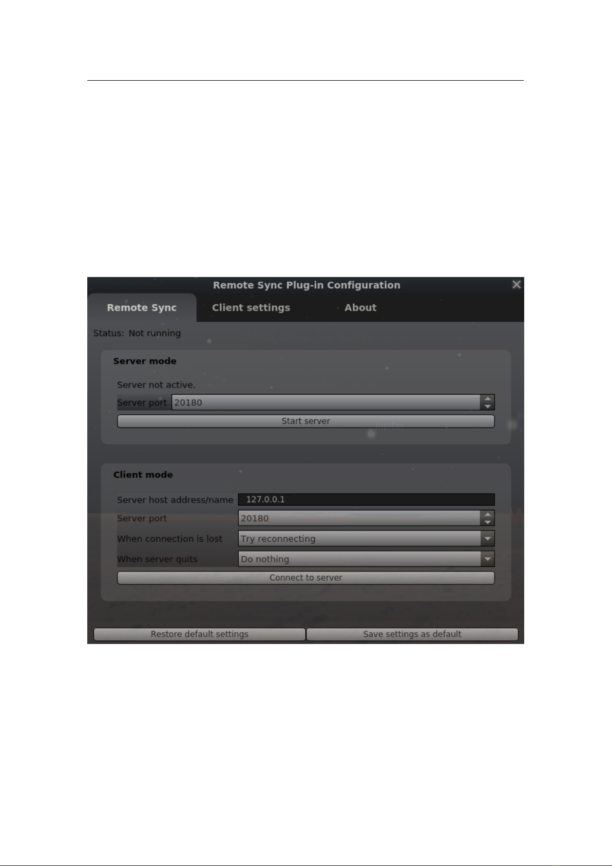
13.6 Text User Interface Plugin 151
8.2 Save current configuration Save the current settings to the main configuration file
8.3
Shutdown Emits a command configured in
13.6.3 Section
[
tui
]
in config.ini file
The section in
config.ini
for this plugin is named only
[tui]
for historical reasons. As always, be careful
when editing!
ID Type Description
tui_font_color R,G,B Font color for TUI text
tui_font_size
int Font size for the TUI
flag_show_gravity_ui
bool
Bend menu text around the screen center. May be useful in
planetarium setups, and should then be used together with
“Disc viewport” in the configuration menu (see 4.3.5).
flag_show_tui_datetime
bool Show date and time in lower center.
flag_show_tui_short_obj_info
bool
Show some object info in lower right, or (in planetarium setups
with “Disc viewport” active,) wrapped along the outer circle
border.
admin_shutdown_cmd
string
executable command to shutdown your system. Best used on
Linux or Mac systems. E.g. shutdown -h now
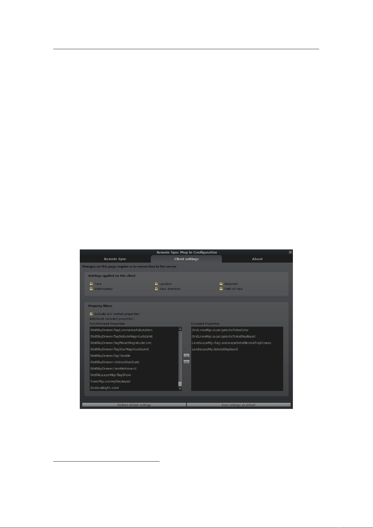
152 Chapter 13. Interface Extensions
13.7 Remote Control Plugin
The Remote Control plugin enables the user to control Stellarium through an external web interface using
a standard web browser like Firefox or Chrome, instead of using the main GUI. This works on the same
computer Stellarium runs as well as over the network. Even more, multiple “remote controls” can access
the same Stellarium instance at the same time, without getting in the way of each other. Apart from system
configuration options, most of the functionality the main interface provides is available through it (Zotti,
Schaukowitsch, and Wimmer, 2017).
The plugin may be most useful for presentation scenarios, hiding the GUI from the audience and allowing
the presenter to change settings on a separate monitor without showing distracting dialog windows. It also
allows to start and stop scripts remotely.
Because the web interface can be customized (or completely replaced) with some knowledge of HTML,
CSS and JavaScript, another possibility is a kiosk mode, where untrusted users can execute a variety of
predefined actions (like starting recorded tours) without having access to all Stellarium settings. The web
API can also be accessed directly (without using a browser and the HTML interface), allowing control of
Stellarium with external programs and scripts using HTTP calls like with the tools wget and curl.
This plugin allows also interfacing other programs with Stellarium.
13.7.1 Using the plugin
Figure 13.9: The default remote control web interface
After enabling the plugin, you can set it up through the configuration dialog. You can configure it to start
the web server automatically whenever Stellarium starts or manually start/stop the server using the “Server
enabled” checkbox or the button
in the toolbar.
The plugin starts an HTTP server on the specified port. The default port is 8090, so you should
reach the remote control after enabling it by starting a web browser on the same computer and entering
http://localhost:8090
in the address bar. When trying to access the remote control from another
computer, you need the IP address or the hostname of the server on which Stellarium runs. On a small tablet,
you may want to use http://myserver:8090/tablet7in.html instead.
The plugin shows the locally detected address, but depending on your network or if you need external
access you might need to use a different one — contact your network administrator if you need help with
that.
13.7.1.1 Password
The access to the remote control may optionally be restricted with a simple password.
13.7 Remote Control Plugin 153
Warning: currently no network encryption is used, meaning that an attacker having access to your
network can easily find out the password by waiting for a user entering it. Access from the Internet to the
plugin should generally be restricted, except if countermeasures such as VPN usage are taken! If you are in
a home network using NAT (network access translation), this should be enough for basic security except if
port forwarding or a DMZ is configured.
13.7.1.2 CORS
The Web API also supports Cross-Origin Resource Sharing (CORS). By enabling CORS, compatible websites
and web apps can be used to control your Stellarium server.
Enable CORS by checking the “Enable CORS for the following origin” option in the configuration
dialog. Then, enter the URL of the website you’d like to use to control Stellarium – e.g.
https://telesc
opius.com. Specify “*” to let any website take control. Do this at your own risk.
13.7.2 Remote Control Web Interface
If you are familiar with the main Stellarium interface, you should easily find your way around the web
interface. The remote control automatically uses the same language as set in the main program. Tabs at the
top allow access to different settings and controls.
Main
Contains the time controls and most of the buttons of the main bottom toolbar. An additional control
allows moving the view like when dragging the mouse or using the arrow keys in Stellarium, and a
slider enables the changing of the field of view. There are also buttons to quickly execute time jumps
using the commonly used astronomical time intervals.
Selection
Allows searching and selecting objects like in section 4.5. SIMBAD search is also supported.
Quick select buttons are available for the primary solar system objects. It also displays the information
text for current selection.
Sky Settings related to the sky display as shown in the “View” dialog as shown in subsection 4.4.1.
DSO The deep-sky object catalog, filter and display settings like in subsection 4.4.4.
Landscape Changing and configuring the background landscape, see subsection 4.4.5
Actions and scripts
Lists all registered actions, and allows starting and stopping of scripts (chapter 17).
If there is no button for the action you want in another tab, you can find all actions which can be
configured as a keyboard shortcut (section 4.3) here.
Location
Allows changing the location, like in section 4.2. Custom location saving is currently not
supported.
Projection Switch the projection method used, like subsection 4.4.4.
13.7.3 Remote Control API
The Remote Control plugin opens many more options from just triggering commands via cronjob to
developing entire alternative GUIs. For a start, you may want to explore the API in a simple SwaggerUI
v 26.3
interface at http://localhost:8090/docs/index.html.
Apart from retrieving quick object info in your browser with e.g.
http://localhost:8090/api/o
bjects/info?format=json&name=Sun
, you can access a running instance of Stellarium with various
programming languages. A few examples:
13.7.3.1 Commandline
It is possible to send commands via command line, e.g.:
curl -d "x =1& y =0.3 " http :// lo c a l host :8 090/ api / main / m ove
wget -- post - data " id = show . ssc " http :// st ella :809 0/ api / script s / run - O / dev / nu ll
curl -d " id= my Script . ssc " h ttp :// localh o s t :80 90/ api / scrip t s / run
curl -d " id= Lan d s c a p e M g r . fogDisplayed & value = f alse " \
http :// localhos t :809 0/ api / st e l p r o p e rty / set
This allows triggering automatic show setups for museums etc. via some centralized schedulers like cron.
To get a complete pretty-printed list of properties and actions, use:
curl -G -d " pro pId = -2& actio n Id = -2" http :// localho s t :809 0/ api / main / sta tus | \
py thon -m js on . tool
13.7.3.2 Node.js
If you want to use node.js to build your own interface app, you may find the following example helpful.
2
It
sets the view direction in one of 3 coordinate systems, depending on the argument:
2
Thanks to user FogoVoar
154 Chapter 13. Interface Extensions
" j2000 " : "[x , y ,z ]" ,
" jNow " : " [ x ,y ,z ] ",
" altAz " : "[x , y ,z ]"
The vector
[x, y, z]
should be a normalized vector (unit length), derived from either J2000.0 or current
equatorial coordinates
(α, δ )
, or from alt-azimuthal coordinates
(Az, alt)
which are however always counted
from south (
[1, 0, 0]
) towards east (
[0, 1, 0]
), with the azimuth
Az
′
counted from South towards East,
Az
′
=
180− Az.
x = cos(
δ)∗ cos(α)
y = cos(
δ)∗ sin(α)
z = sin(
δ)
x = cos(alt)∗ cos(Az
′
)
y = cos(alt)∗ sin(Az
′
)
z = sin(alt)
const url = ’ http ://192 . 1 6 8 . xxx .xxx :8090 / api / main / view ? j200 0 =[0.5 ,0.3 ,0.2] ’;
fetch (url , {
me thod : ’ POST ’ ,
he a ders : {
’ Content - Type ’: ’ a p p l i c a t i o n / json ’
}
})
. then ( respo n s e = > {
res p onse . text (). then ( text = > c o nsole . log (’ Raw respons e : ’, text ));
re turn res p onse . json ();
})
13.7.3.3 Python
An example for time control:
im port req u ests
STELLARIUM_URL = ’ http ://1 9 2 . 1 6 8.1. 1 0 0 : 8 090 / api /main ’
def set_time ( julian_d ay , timerat e ):
url = f"{ STELLARIUM_URL }/ time "
data = " time ="+ str ( julian_d a y )+ " & t i merate =" +str ( t i merate )
print (f " Reque s t URL : { url }" )
print (f " Reque s t Data : { data }" )
try :
res p onse = r equests . post ( url , data = data )
print (f " Respons e S tatu s Code : { respons e . status_ c o d e } " )
print (f " Respons e C ontent : { respo n se . text }")
res p onse . ra i s e _ for_stat u s ()
if re sponse . text . str ip () == " ok" :
re turn {" status " : " succe ss " , " mes sage ": " Time set s u c c e s s f u l l y " }
else :
re turn {" status " : " error ", " messag e " : r esponse . text }
ex cept req u ests . exceptions . Re q u e s t E x ception as e:
print (f " Err or set t ing time : { e } ")
re turn {" status " : " error ", " messag e " : str (e )}
13.7.4 Developer information
If you are a developer and would like to add functionality to the Remote Control API, customize the web
interface or access the API through another program, further information can be found in the plugin’s
developer documentation
3
.
13.7.5 Acknowledgements
This plugin was created by Florian Schaukowitsch in the 2015 campaign of the ESA Summer of Code in
Space
4
programme.
If you are using this plugin in your scientific publications, please cite Zotti, Schaukowitsch, and Wimmer
(2017).
3
https://stellarium.org/doc/head/remoteControlDoc.html
4
https://socis.esa.int/
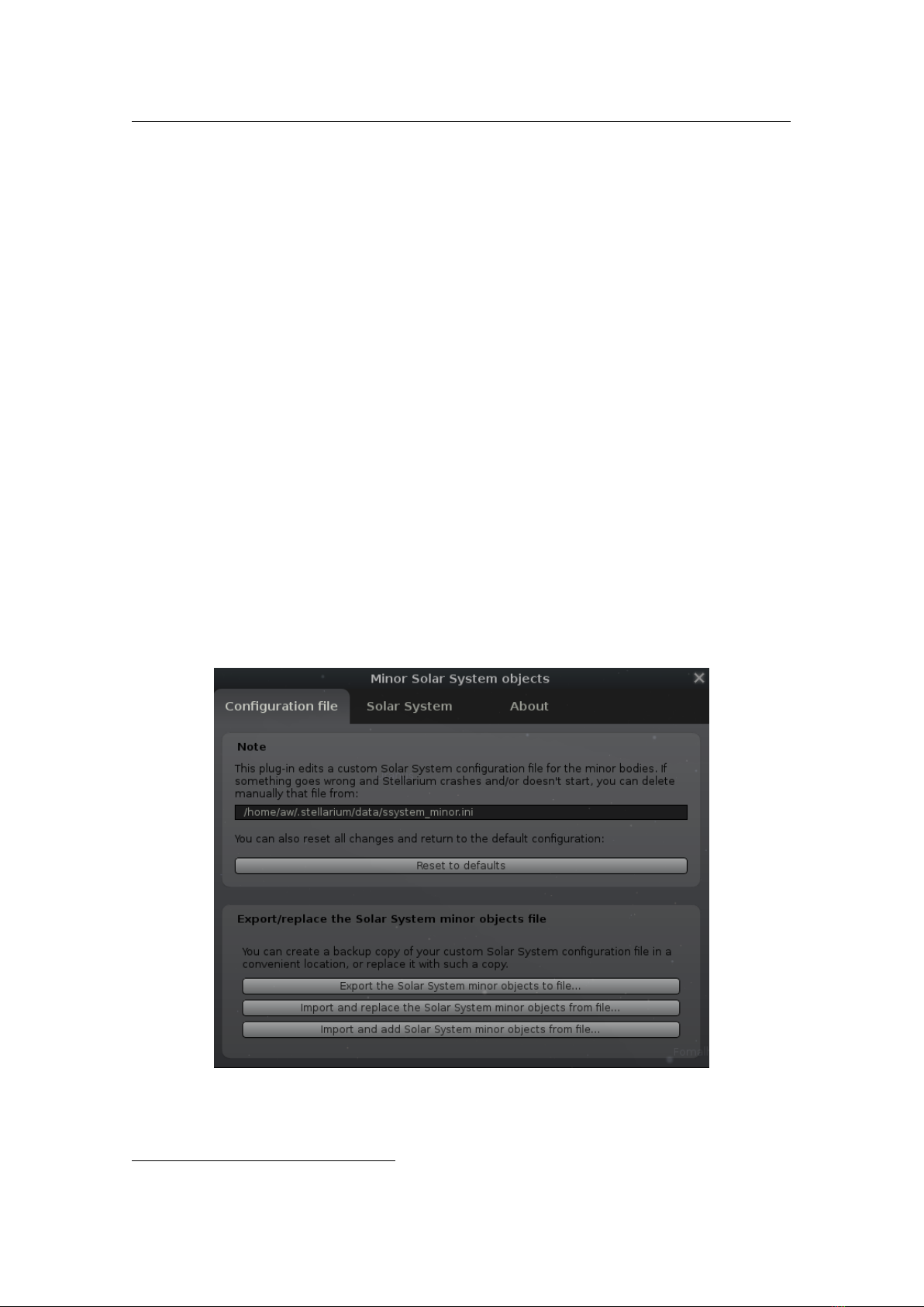
13.8 Remote Sync Plugin 155
13.8 Remote Sync Plugin
The Remote Sync plugin enables setups which connect several instances of Stellarium running on a network.
This may be useful in installations where one presenter wants to allow a larger audience to follow the actions
on several dim screens (e.g., when you need to avoid a projector’s bright light in a public observatory).
The actions performed on a “master” instance, which acts as a server, are automatically replicated on all
connected clients. These clients may run on the same device the server runs, or may access the server over a
network.
The plugin is still quite experimental, but is provided for testing and developing purposes. You can
configure it through the standard plugin settings dialog (Figure 13.10). One Stellarium instance can either
run in the server mode or connect to an existing server as a client. A custom TCP protocol is used for the
connection. The port used by the server is configurable, and the clients must know the IP address or host
name and the port of the server.
Figure 13.10: RemoteSync settings window
Alternatively, you may start the plugin through command line arguments. This is useful for automated
setups or when multiple instances are running on the same computer. To start the instance as a server, use
the
--syncMode=server
argument with the optional
--syncPort
parameter to specify the port to listen
on. To start a client instance, use
--syncMode=client
and use
--syncHost
and
--syncPort
to specify
the server to connect to.
In the settings window, you can also specify what should happen when the client loses the connection to
its server, and what to do when the server quits normally. You can choose between
Do nothing:
connection is lost and will not be re-established. Stellarium client keeps running in whatever
state it was, waiting for keyboard/mouse interaction.
Try reconnecting:
Assume Stellarium is switched off on the server but may come back online again, or
assume some temporary network problem. Stellarium client just keeps running in whatever state it
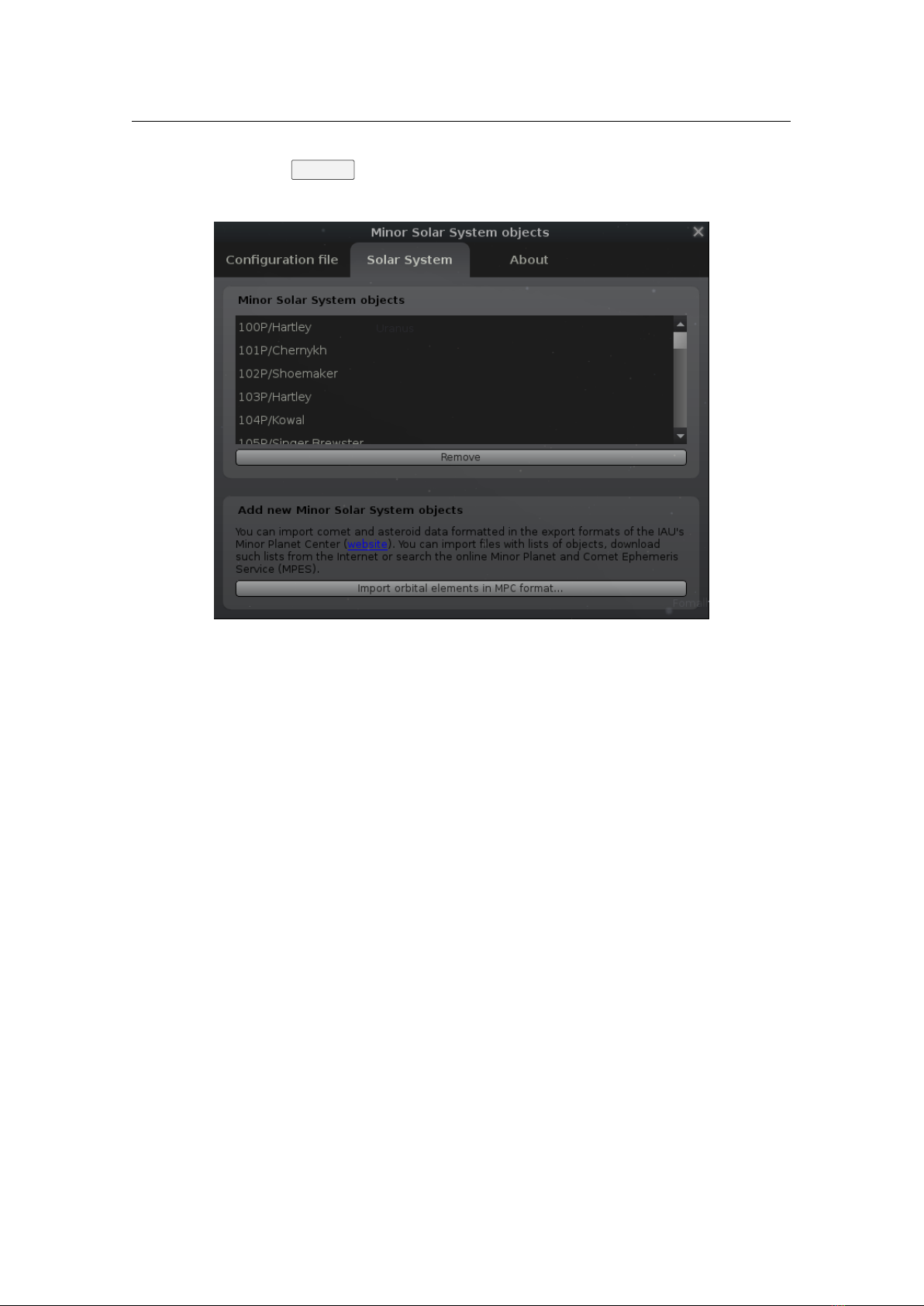
156 Chapter 13. Interface Extensions
was, but tries to reconnect.
Quit:
Assume the server always runs until switched off at the end of operating hours. This is intended for
pure client screens without keyboards. When the server is shut down, assume this is the end of the
day, and exit Stellarium. An enclosing run script can then shutdown the client computer before power
is switched off with some main switch.
By default, the following things are synchronized:
•
simulation time
•
viewer location
•
the selected object
•
view direction
•
current field of view
•
all StelProperty-based settings except for GUI-related properties. This includes almost all settings
visible in the configuration dialogs such as projection type, sky and view options, landscape settings,
line colors, etc.
Because there is currently no full time synchronization implemented, for the best results all client computers
should make sure their system clocks are set as close as possible to the server computer’s clock (preferably a
few milliseconds difference at most). This can be done for example by using an NTP server.
5
If all your
Stellarium instances run on the same device, this is of course not necessary.
Figure 13.11: RemoteSync client settings window
It is also possible to exclude some state from being synchronized. On each client, the client configuration
GUI (Figure 13.11) allows to disable specific settings from being synchronized on this client.
The lower part of this dialog allows you to fine-tune which named StelProperties (which hold parts
of the internal program state) should be excluded from synchronization. The configuration dialog lists all
available properties which usually have easy to understand names on the left side. Highlight one or more
properties which you don’t want synchronized and press the arrow button to move them to the list of excluded
properties.
For historic reasons there are two kinds of Properties: Actions (Boolean switches, for which also hotkeys
can be assigned) and (genuine) StelProperties. The latter have names indicating which module they belong
to and may have other data types (numbers, colors, . . . ). Note that the actions frequently are just alias names
of Boolean StelProperties, so in order to inhibit a certain property from being synchronized, you must find
5
Instructions on how to use the public NTP server pool for the most common operating systems can be found at
https://www.pool.ntp.org/en/use.html.
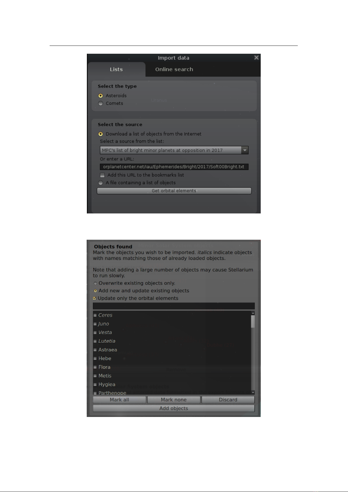
13.8 Remote Sync Plugin 157
both entries.
Properties of plugins will only be visible when the respective plugin has been enabled. When a plugin
has been disabled, its properties may vanish from the stored list of non-synchronized properties.
Each client can have different settings. This could allow installations with several screens where on one
screen you show the constellation figures, another screen shows the distribution of deep-sky objects in the
same frame, and a third screen may show a close-up view of the currently centered object. Or just show
several sky cultures, or show the sky at different locations, . . . .
The names of all available StelProperties from which you might want to select a few to exclude from
synchronisation can also be found with a little scripting (see chapter 17). Open the script console
F12
and
enter the following call:
core.output(core.getPropertyList());
Run the script and inspect the output tab. It may take a little guesswork to select the right names, but the
general structure of property names like
<Module>.<Property>
should help you to find your way around.
13.8.1 Developer notes
Usually the synchronisation fails if you attempt to use different versions of Stellarium. You can override this
behaviour with an entry in the respective section of config.ini:
[ Re m o teSync ]
allowVe r s i o n M isma t c h = true
13.8.2 Finetuning
This plugin makes use of the QLoggingCategory infrastructure. By default it is very verbose and prints each
transmitted property to the logfile. To reduce verbosity when it works, configure an environment variable
with these entries (Note the closing semicolon!):
QT_LOGGING_RU L E S = " stel . plugin . remo t e S y n c . debu g = true ;
stel . plugi n . re m o t eSync . client . debug = fal se ;
stel . plugi n . re m o t eSync . protocol . debug = false ;"
The final parts may be debug|info|warning|critical = true|false. Default: true.
Author and Acknowledgements
This plugin was created mostly by Florian Schaukowitsch in the 2015-16 campaigns of the ESA Summer of
Code in Space
6
programme.
6
https://socis.esa.int/

158 Chapter 13. Interface Extensions
13.9 OnlineQueries Plugin
Stellarium includes and provides lots of information about many kinds of objects. However, there are
scientific websites which provide even more specialized information about particular objects. This plugin
(Zotti, S. M. Hoffmann, et al., 2023) allows online access to several websites on a variety of special topics.
To retrieve information, select the first tab and press the respective button labeled with the information source.
The result is displayed in a browser view
7
.
Wikipedia
The free online encyclopedia provides information about many bright stars, the planets, moons
and many asteroids, as well as many deep-sky objects. The lookup is based on the English proper
name.
AAVSO
The International Variable Star Index
8
of the American Association of Variable Star Observers
(AAVSO) provides data about variable stars.
GCVS
The General Catalogue of Variable Stars
9
of the Sternberg Astronomical Institute and the Institute
of Astronomy of the Russian Academy of Sciences in Moscow.
ASE
The All Skies Encyclopaedia
10
of the IAU Working Group on Star Names (WGSN) which collates and
collects the data on cultural names of stars and constellations in order to preserve their heritage and
distribute the knowledge about them beyond their culture of origin.
In addition, you can configure up to three further websites. These must provide some public website
which takes a query for a Hipparcos star number or object name.
Regardless of the current program language, the result is always presented in English or the language of
the respective website.
13.9.1 Section
[
OnlineQueries
]
in config.ini file
You can edit the
config.ini
file to change settings of the OnlineQueries plugin. The only strings you
should need to touch are the
customN_...
entries (
N ∈ {1, 2, 3}
). The placeholder
%1
will be filled by either
the Hipparcos number (if the respective
customN_use_hip
is
true
) or by the first English name used in
Stellarium. The
customN_use_hip
should be
true
to use a star’s Hipparcos number, or
false
to use the
English name as key.
ID Type Default
aavso_hip_url string (don’t override)
aavso_oid_url
string (don’t override)
ase_url
string (don’t override)
gcvs_url
string (don’t override)
wikipedia_url
string (don’t override)
custom1_url string
custom2_url string
custom3_url string
custom1_use_hip boolean true
custom2_use_hip
boolean true
custom3_use_hip
boolean true
disable_webview boolean false
7
For technical reasons, on some platforms the result is displayed in the system’s default web browser. On some
other platforms, e.g. Windows/WSL with Ubuntu or some ARM computers, the web view fails to work properly. On
these platforms you should manually edit config.ini and set the disable_webview entry in the config file.
8
https://www.aavso.org/vsx/
9
http://www.sai.msu.su/gcvs/
10
https://ase.exopla.net/index.php/All_Skies_Encyclopaedia

13.10 Sky Culture Maker Plugin 159
13.10 Sky Culture Maker Plugin
LUCA-PHILIPP GRUMBACH, SUSANNE M. HOFFMANN
13.10.1 Introduction
To ease the creation of sky cultures (Chapter 9) and avoid mistakes caused by the shortcomings of manual
coding, Stellarium in 2025 started developing a “Sky Culture Maker” (SCM) plugin. It provides the technical
means of visually creating a new sky culture, allowing the user to interact with the usual Stellarium star
map while drawing constellation stick figures and attaching artwork in a wizard-like editor. The SCM
also prompts the user to supply copyright and category information, geographical schema, and all other
requirements for a well-defined sky culture.
With the many new sky culture features released in 2025 (a new data format, display options for historical
frames of reference, and audio output of sky culture information) the requirements on both the data files and
the accompanying description have grown a lot. The SCM is intended to handle these details for the user and
provide an intuitive UI.
However, beware that the plugin is still in development. It was originally set up as a student project
in a software development course, but tests with students from the humanities and researchers in cultural
astronomy showed that it is already useful for users who are comfortable editing source code. Future versions
will continue to improve the SCM.
13.10.2 Getting Started
Figure 13.12: SCM plugin: start dialog
The SCM plugin is disabled by default. In order to use it, you will need to activate it first according to
section 12.1. Once activated, a toolbar button will appear. This button is also an indicator of whether
the SCM is currently open: pressing it toggles the icon to a glowing version and opens the start dialog shown
in Figure 13.12.
The Create button opens the main dialog where you can build a new sky culture. If the Sky Culture
Converter was enabled at build time, a Convert button also appears (see section 13.10.3 for details). The Edit
button opens a file chooser where you can select an existing sky culture. It will be loaded into the SCM for
editing.
13.10.3 Converting an Existing Sky Culture
The SCM includes a UI for the Sky Culture Converter (section 9.4) that transforms legacy sky cultures using
the old .fab format into the new JSON-based format (Chapter 9).
Build-time requirement
The converter is not built by default. To enable it, pass
-DSCM_SHOULD_ENABLE_CONVERTER=ON
to CMake
when configuring the build. The converter requires Qt 6 or later and it is automatically disabled for Qt 5
builds and Windows ARM64 targets. It also depends on Tidy HTML, GNU gettext, and zlib. CMake will
download the converter library automatically via CPM.
Using the converter
When the converter has been built, a Convert button appears in the SCM start dialog alongside the Create
button (Figure 13.13).
1. Press Convert in the start dialog.
2.
A file chooser opens (Figure 13.13, panel b). Select an archive that contains the old sky culture
files. Supported formats:
.zip
,
.rar
,
.tar
,
.7z
. Selecting a plain directory is not supported by the
converter. Note that only plain
.tar
archives are supported. Compressed variants such as
.tar.gz
or .tar.bz2 are not.

160 Chapter 13. Interface Extensions
(a) Start dialog with Convert button (b) Converter file chooser
Figure 13.13: SCM plugin: converter workflow dialogs
3.
The converter processes the archive and writes the resulting files directly into Stellarium’s
skycultures
directory. If the application does not have write permission there, a dialog prompts you to choose an
alternative output folder.
Note: Sky culture identifiers are case-sensitive. For example,
chinese_chenzhuo
and
chinese_Chenzhuo
are treated as different cultures.
13.10.4 Creating a New Sky Culture
After pressing Create in the start dialog, you will be greeted by the Overview tab of the main dialog
(Figure 13.14, panel a). This dialog is different from most dialogs in Stellarium, as it is an independent
window that can be moved outside the Stellarium application, including onto a second monitor for more
workspace. To resize it on Windows, you must drag the tiny square handle in the bottom-right corner.
Note: Because the dialog is an independent window, it may open behind the Stellarium main window and
therefore not be immediately visible. If nothing seems to have happened after pressing Create, the dialog
has most likely opened in the background or on another monitor. Try clicking once on the Stellarium main
window to bring the SCM dialog to the front. If that does not work, try minimizing the Stellarium main
window. The same behaviour applies to the Constellation Editor described in section 13.10.5. In the first
text input, you may enter a name for your new sky culture. This field is mandatory. Below the name field is
the constellation list, which is empty until you create constellations (see section 13.10.5). Before doing that,
it is worth browsing the remaining tabs.
Description tab
The Description tab (Figure 13.14 b) collects textual information about the sky culture. It contains dropdown
menus as well as mandatory (marked with an asterisk) and optional text fields. Scroll through all fields and
supply as much information as possible. Your inputs are used to generate the sky culture description file
(
description.md
), which Stellarium will use to display certain information to users. For details on the
expected content and structure of this file, see section 9.1.
Common Names tab
The Common Names tab (Figure 13.14 c) manages culture-specific names for stars, planets, and deep-sky
objects.
The table at the top lists the common name entries you have already created. The input fields below are
used to enter new names. In order to automatically fill in the type, identifier, and English name, select an
object in Stellarium and press Copy Data From Selected Object. The mandatory fields are marked with an
asterisk, just like in the Description tab.
Note that in some cultures, planets carry different names depending on the time of day. The Visible
dropdown lets you choose whether a name is always visible, or only during morning or evening. For
non-planetary objects the value is fixed at Always visible.
For the full specification of common names for stars, planets and deep-sky objects, see sections 9.2.7,
9.2.7.3, and 9.2.8.
Workflow for managing entries:
•
Add: Fill in the fields and press Save As New Entry. The fields are cleared afterwards.
•
Edit: Select a row in the table; the fields are populated with the current values. Make your changes
and press Update Selected Entry.
•
Remove: Select a row and press Remove Selected Entry. This action is irreversible!
Location tab
The Location tab (Figure 13.14, panel d) specifies where and when the sky culture was or is practiced.

13.10 Sky Culture Maker Plugin 161
(a) Overview tab (b) Description tab
(c) Common Names tab (d) Location tab
Figure 13.14: SCM plugin: main dialog tabs for creating a sky culture
(a) Drawing tab (b) Information tab (c) Artwork tab
Figure 13.15: SCM plugin: Constellation Editor tabs and drawing workflow

162 Chapter 13. Interface Extensions
The upper part of the tab shows a world map, which allows you to digitize the geographic territory of
the culture by drawing polygons. Simply click on the map to register corners and extend the polygon.
•
At least one polygon is required before exporting the sky culture. You can later edit or refine the
GeoJSON format in your GIS applications.
•
Hold
and drag with the left mouse button to move the map while drawing.
•
Press
Ctrl
+
Z
to undo the last click.
•
Press
Esc
to discard the entire current polygon.
•
Double-right-click to finish the polygon. A dialog then asks for the start and end year during which
the culture was or is practiced. The special value 9146 indicates that the culture is still practiced.
•
A short help summary for all map interactions is available by clicking the ? button in the bottom-right
corner of the map.
Instruction for creating geo-polygons: The polygons are meant to indicate the origin of the astronomical
culture that is represented in Stellarium. We regard this information as educational in terms of understanding
the reasons for the selection of specific images, because the specific fauna and flora, and the geological
features of the area influence cultural habits (astronomy is used for forecasting seasonal weather, encounters
with migrating birds, fish, and other animals that might be depicted in the constellations). For that reason,
the polygons of historical indigenous settlements or the extent of empires are more important than modern
borders of states or enclosures. For instance, in a modern state (like the USA) there might be reserves for
indigenous nations (e.g. the Navajo), but for our purpose these legal boundaries are less important than the
original area where their sky cultures had been developed in pre-Columbian America.
Note the Time Slider! You have the option to simulate the movement of a culture over time. For instance,
the Indian Vedic culture developed in the Indus Valley first, then spread to the Ganges Plateau and then to
the entire Indian subcontinent (and with Hinduism even beyond). So, we defined three time steps for the
Indian Vedic culture with different geographical extents. This may help in understanding both where any
specific culture is practiced today and where it stems from.
Note that the time slider does not affect the display in the Stellarium main simulation, i.e. the display of the
sky. It is only meant to illustrate the evolution of cultures.
The polygon data is then saved to a
territory.geojson
file. For details on its format see section 9.3.
For information on geoscheme regions, see section 9.2.1.
13.10.5 Creating a New Constellation
Head back to the Overview tab and press Add Constellation to open the Constellation Editor (Figure 13.15,
panel a). This editor consists of three tabs.
Drawing tab
The Drawing tab lets you draw constellation lines directly on the Stellarium sky map (see also section 9.2.4
for the underlying data format).
1. Press the Pen button to activate drawing mode.
2. Hover over a star and a snapping indicator will show you which star is currently targeted.
3. Right-click on the star to set it as the start of a line segment.
4.
Move the mouse to the next star; right-click again to complete the segment and immediately begin the
next one from that point.
5. To stop drawing, double-right-click or simply press the Pen button again.
Using this workflow you can build complex stick figures (see Figure 13.16 a). Mistakes can be undone with
the Undo button (one segment at a time) or erased with the Eraser tool: press Eraser, then hold the right
mouse button and drag through any line segment to remove it.
Information tab
The Information tab (Figure 13.15 b) records metadata about the constellation. The English name and the
unique identifier are mandatory; all other fields are optional but recommended. A possible identifier is
generated automatically from the English name, but you may change it manually as well.
Artwork tab
The Artwork tab (Figure 13.15 c) lets you attach an illustration to the constellation. For background on
artwork and its role in sky cultures, see section 9.2.4.1.
Press Upload Image and select an image file. Three blue anchor points appear on the image. To align
the artwork with the sky:
1. Select an anchor point in the tab.
2. Select a star in Stellarium (for example, one that appears in the constellation).
3. Press Bind Star to associate that star with the anchor point.
13.10 Sky Culture Maker Plugin 163
4. Drag the anchor point to the position in the image that the star represents.
5. Repeat for the remaining anchor points.
An example result is shown in Figure 13.16. If the image is not visible on the sky map, try repositioning the
anchor points. The SCM does not draw images that become too distorted.
(a) (b)
Figure 13.16: Example constellation drawing (a) in progress and (b) with artwork aligned
Dark constellations
The Overview tab also offers Add Dark Constellation. The dark constellation editor works just like the
regular editor, except that lines are not snapped to stars. You may click anywhere in the sky to place a vertex
using its sky coordinates directly. See section 9.2.4 for details on dark constellations.
Managing constellations
When you save a constellation, it is added to the list in the Overview tab (Figure 13.17). Select a constellation
in the list to Edit or Remove it.
Figure 13.17: SCM plugin: Overview tab with two example constellations
13.10.6 Exporting the Sky Culture
When the sky culture is ready, select a license from the dropdown menu in the Overview tab. For guidance
on which license to choose, see section 9.1.3. Then press Export Sky Culture. If any mandatory fields are
incomplete, an error message identifies what is missing. Otherwise the Export Dialog (Figure 13.18) opens.
Read through the checklist items and confirm you have followed them. The checkbox Merge constellation
lines into polylines on export (checked by default) merges consecutive line segments that share an endpoint:
for example,
[1,2]
and
[2,3]
become
[1,2,3]
in the JSON output, producing a cleaner file. It is
recommended to leave this option enabled.
Choose Export to export while keeping the SCM open, or Export and Exit to export and close the plugin.
The export creates a folder containing:
•
index.json — see section 9.2
•
description.md — see section 9.1

164 Chapter 13. Interface Extensions
Figure 13.18: SCM plugin: Export dialog
•
territory.geojson — see section 9.3
•
illustrations/ — sub-folder with any uploaded artwork images
13.10.7 Closing the Plugin
Press the X icon in a dialog’s title bar or Cancel wherever available. This opens the dialog shown in
Figure 13.19, offering three choices:
Figure 13.19: SCM plugin: Close dialog
Hide editor
Hides all SCM windows but preserves all data. Reopening the SCM via the toolbar button
restores the previous state.
Close without saving Shuts down the SCM plugin and discards all unsaved data.
Don’t close Returns to the SCM without any changes.
Section
[
SkyCultureMaker
]
in config.ini
The following settings can be adjusted manually in the
config.ini
file under the
[SkyCultureMaker]
group. Colors are given as comma-separated R,G,B values in the range 0–1.
Key Type Default
fixedLineColor float R,G,B 1.0,0.5,0.5
fixedLineAlpha float 1.0
floatingLineColor
float R,G,B 1.0,0.7,0.7
floatingLineAlpha float 0.5
maxSnapRadiusInPixels
int 25
mergeLinesOnExport
bool true
Key descriptions:
fixedLineColor / fixedLineAlpha
Color and opacity of constellation line segments that have been commit-
ted (drawn with right-click).
floatingLineColor / floatingLineAlpha
Color and opacity of the preview line segment following the cursor
while drawing.
maxSnapRadiusInPixels
Maximum distance in screen pixels within which the cursor snaps to the nearest
star or DSO.
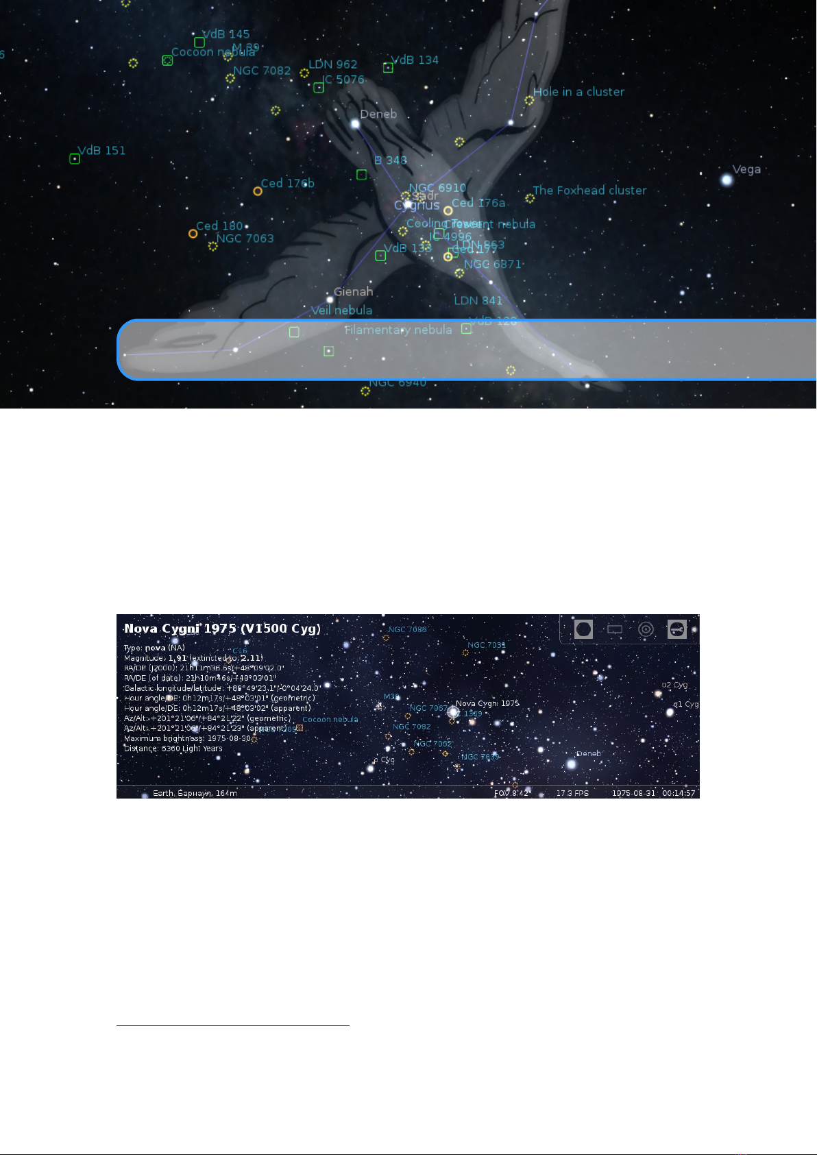
13.10 Sky Culture Maker Plugin 165
mergeLinesOnExport
Whether consecutive line segments sharing an endpoint are merged into polylines
on export (mirrors the checkbox in the export dialog).
13.10.8 Further Development
The plugin is still in active development. In its current state it provides the fundamental features but is not
yet fully functional (beta). If you test the wizard, please report missing features or bugs via the Stellarium
issue tracker.
13.10.9 Acknowledgments
Fabian Hofer, Vincent Gerlach, Luca-Philipp Grumbach, Richard Hofmann, and Mher Mnatsakanyan
developed this plugin in 2025 at the University of Jena, under the supervision of Jan Heinrich Merker and
with Susanne M. Hoffmann as product owner.
If you use this plugin in scientific publications, please cite this User Guide and Zotti, Kabatsayev, et al.
(submitted).

166 Chapter 13. Interface Extensions
13.11 Solar System Editor Plugin
Stellarium stores its data (orbital elements and other details) about solar system objects (planets, their moons,
minor bodies) in two files. File
data/ssystem_major.ini
in the installation directory contains data for the
planets and their moons, and should never be touched by users. File
data/ssystem_minor.ini
contains
data for minor bodies, i.e., planetoids and comets. The file will be taken from the user data directory if it also
exists there, which means that users can add minor planets or comets as they become observable by editing
this file.
The orbits of minor bodies (minor planets and comets) are specified with orbital elements for Kepler
orbits (after JOHANNES KEPLER (1572–1630) who found the true shape of the orbit of a small body around
a large one being a conic section, i.e., circle, ellipse, parabola or hyperbola). These elements describe the
instantaneous shape and orientation of the object’s orbit around the Sun at a particular time called the epoch.
We compute positions from these osculating elements of minor body orbits, but the result is only valid for a
moderately short timespan around the epoch, because the major planets can exert noticeable gravitational
perturbations on the objects when they come close, and so these orbital elements, which are mere snapshots
in time, need to be updated on a regular basis. Stellarium does not perform numerical integration that could
work out the orbital changes automatically, and so the element file needs to be modified to compute positions
further away from the orbit’s epoch. See Appendix D.2 for more details, and see e.g. Meeus (2007) for a
discussion of a few interesting examples of orbital development. When you go out hunting for asteroids and
comets, this plugin is for you.
This plugin provides access to the Minor Planet Center (MPC
11
) server where the latest Solar System
information can be found. When this plugin is loaded (see section 12.1) and you open the configuration
dialog, the first tab allows to import, export or reset your
ssystem_minor.ini
, and also to load extra
data for minor bodies in Stellarium’s
.ini
format. For example, the installation directory contains a file
ssystem_1000comets.ini
which contains data for over 1000 historical comets. Currently it is not possible
to select only a few from that, so try loading this only on a reasonably fast computer, and think about deleting
comets again (or resetting the file) when you don’t require them.
Figure 13.20: Interface of Solar System Editor plugin: Configuration file tab
The second tab lists all currently loaded minor bodies (see figure 13.21). It is recommended to remove
old entries of yesteryear’s comets if you don’t need them any longer. Just select one or more objects and
press
Remove
. If you have a very weak computer, you may want to reduce the number of minor bodies to
11
https://www.minorplanetcenter.net
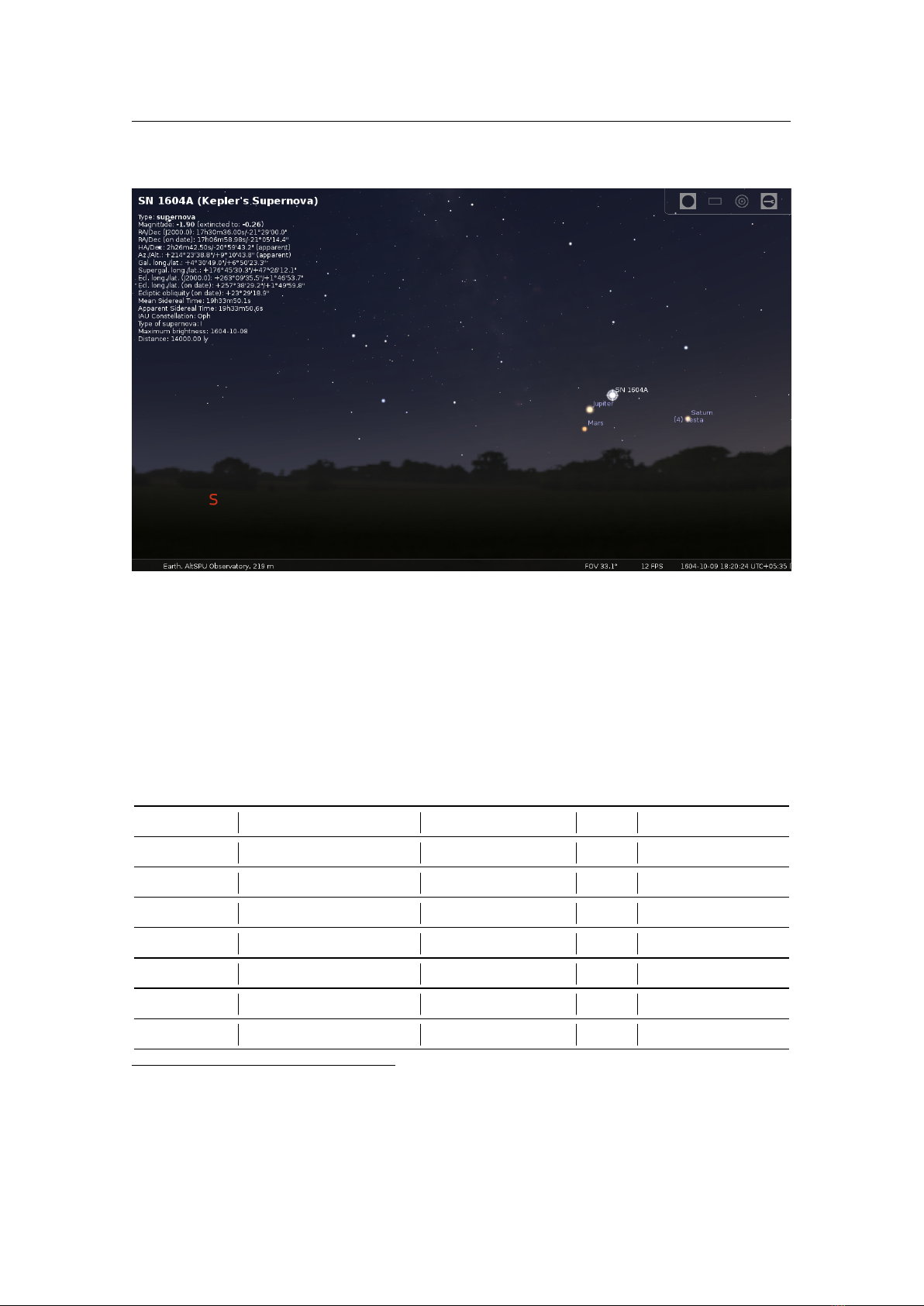
13.11 Solar System Editor Plugin 167
just a handful to improve performance.
Figure 13.21: Interface of Solar System Editor plugin: Solar System tab
On this tab, you also find the option to connect to the MPC and download current orbital elements, or
load a text file in the format provided by MPC (see figures 13.22 and 13.23).
Once MPC data has been downloaded, the user can select objects for updating the user’s
ssystem_minor.ini
.

168 Chapter 13. Interface Extensions
Figure 13.22: Interface of Solar System Editor plugin: Import data dialog
Figure 13.23: Interface of Solar System Editor plugin: Import data dialog — view after downloading
and parsing the MPC data.
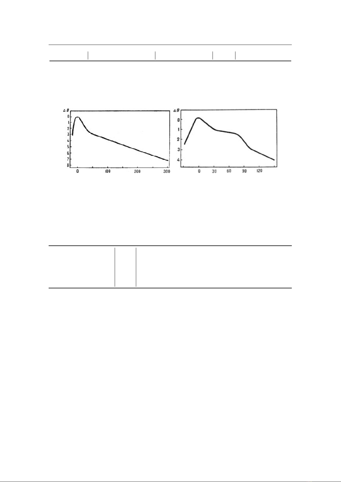
13.12 Nebula Textures Plugin 169
13.12 Nebula Textures Plugin
The Nebula Textures plugin allows users to customize deep-sky object (DSO) textures, precisely rendering
them in Stellarium like default textures. Astronomy amateurs can use it to create a collection of their own
astrophotography, visual-like sketches, paintings, and even more in Stellarium. It also serves as a simple
client for Astrometry.net, enabling blind-solving and precise positioning of astronomical images. The
plugin’s full functionality includes online plate-solving and positioning of astronomical images, as well as
the management and rendering of custom textures.
13.12.1 Online Solving and Texture Management
Instructions for integrating astrophotography images via online plate solving.
1.
Prepare an Image: Prepare a processed rectangular bitmap file of a deep-sky object, in a format
that supports both Astrometry analysis and rendering, such as PNG, JPG, TIF, or GIF. You should
adjust the image background brightness to suit Stellarium by referencing the nebulae images in the
Stellarium
nebulae/default
directory. Typical astrophotography images with TAN projections are
fine, but avoid images with high field distortion. If the image’s FOV is too large, it is recommended
to manually split it into multiple sub-images beforehand. Ensure that the image is not flipped
horizontally or vertically!!! It’s recommended to use a descriptive ID or nickname as the filename.
While Nova Astrometry does not strictly limit image size, keeping it below 20 MP ensures efficient
plate solving.
2.
Open Image: By default, the plugin opens the “Solve and Add” page. Click the
Open File
button to
select an image file or paste the file path into the “Image Filepath” text box.
3.
Enter API Key: Paste your Astrometry API key into the corresponding text box (password mode by
default). If you don’t have one, click
Astrometry API key
to obtain it after registering or logging in.
Check
2 Remember me
to store the key for future use.
4.
Upload and Solve: Click
Online Solve
to begin uploading and solving the image. Ensure system
proxies are disabled to avoid errors. The solving process may take seconds to minutes, depending on
the Astrometry.net server. If you need to stop the solving process, click the
Cancel
button.
5.
View Solving Results: After successful solving, the image’s center and corners’ J2000 equatorial
coordinates (in decimal degrees) will be displayed.
6. Optional Testing:
•
Click
Goto Center
to locate the texture’s center.
•
Use
Test this texture
to preview the texture. If it overlaps with default textures, you should
check
Disable default textures
to avoid visual conflicts. The
Test this texture
button will toggle
between “Test this texture” and “Stop test” to start and stop the rendering process. Remember
to click
Stop Test
afterward to restore the rendering of the default nebula textures!
•
When testing is active, modifying the coordinate spinboxes (including using the mouse wheel)
will immediately update and redraw the texture in real-time, enabling an interactive experience
for fine-tuning alignment.
•
For images solved via Astrometry.net, if manual coordinate adjustments deviate too much,
Reset
will appear. Click it to reset the coordinates back to the original astrometric solution.
•
The dropdown menu is used to adjust texture brightness, with three options: Bright, Normal,
and Dark. The default Normal setting is suitable for most cases.
•
You can repeatedly press the
s
key in the main view to toggle star visibility and verify whether
the image is aligned accurately.
7.
Add Texture to Storage: Click
Add the Texture to Custom Storage
to permanently save the texture.
The original image will be copied to Stellarium’s plugin folder in the user directory. After adding a
texture, you should restart Stellarium to fully integrate the texture into the module.
8.
Display Settings: After restarting Stellarium, switch to the
Custom Textures
page of the plugin to
manage your custom textures. Options include
Show Custom Textures
(showing/hiding textures),
Avoid Area Conflict
(avoiding overlaps with default textures), and
Reload
(reloading custom tex-
tures).
9. Locate a Texture: Double-clicking a texture item in the list will center the view on that texture.
10.
Remove a Texture: To remove a texture, switch to the
Custom Textures
page, select it in the list
view and click
Remove selected item in Custom Textures
. The configuration file will update, and the
corresponding image file in the plugin folder will be deleted. However, Stellarium may continue
rendering the texture until it is restarted.

170 Chapter 13. Interface Extensions
13.12.2 Manual Texture Addition)
Instructions for adding manual textures (e.g., sketches, paintings). The process is similar to the one above,
but performing online solving is not required:
•
Open the image file. Stars in non-astrophotographic images may not align precisely with the software’s
stars, so it is recommended to use the texture without stars (de-star it).
•
Input the J2000 equatorial coordinates (in decimal degrees) for the image corners, aligning with the
bitmap display.
•
If needed, use an astrophotography image with a similar field of view (FOV) to obtain approximate
corner coordinates via online solving first. Alternatively, enable Digitized Sky Survey layers in
Stellarium (Disable constellation lines, illustrations, grids, and other unrelated elements to approximate
a realistic effect), adjust the field of view and rotation to match the texture, and capture a screenshot
for solving. After obtaining the solved coordinates, replace the image path with the texture path.
•
Then, debug and render the texture, adjusting coordinates until the texture stars align accurately with
Stellarium stars. Finally, add the texture to the custom storage.
13.12.3 Notes
1.
All uploaded images are automatically assigned a CC BY-NC-ND 3.0 license by Astrometry.net and
are not publicly visible by default. Avoid excessive uploads to prevent server congestion or issues
with your API key.
2.
After adding a texture, you must restart Stellarium to fully integrate the texture into the module. The
same applies when deleting a texture.
3.
To back up your texture library or share it with others, copy the plugin folder from your user config
directory. You can find the exact plugin storage path in the “About” section of the plugin GUI. For
Windows systems, this path is usually something like:
%APPDATA%\Stellarium\modules\NebulaTextures
You can then share this folder with others, and they can place it in the same directory on their system
to use the custom textures.
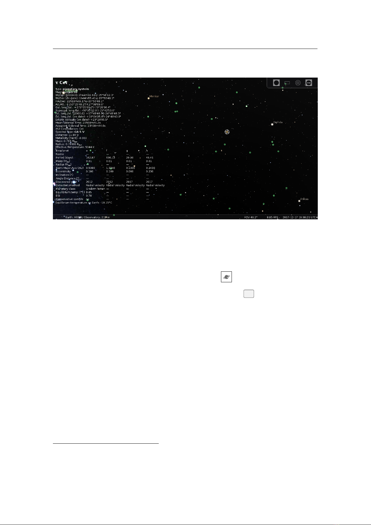
13.13 Calendars Plugin 171
13.13 Calendars Plugin
GEORG ZOTTI
13.13.1 Introduction
The calendar dates in the main program behave like most other astronomical software titles:
•
Dates are given in the Gregorian calendar for all dates beginning with October 15, 1582.
•
All earlier dates are given in the Julian Calendar in its finalized form by AUGUSTUS. Historically,
only dates beginning with March 1st, 4 A.D. coincide with historically recorded dates: the Roman
priesthood messed up the 4-year count introduced by JULIUS CAESAR and counted leap years every
third year. AUGUSTUS decreed to omit leap days from 12 B.C. to 4 A.D. to move the seasons to
where JULIUS CAESAR had placed them.
•
Given the errors in the Julian calendar, simulation in early prehistory will provide non-intuitive
calendar dates for the seasons’ beginnings.
•
Astronomical counting of years includes a year zero and negative years. Historical calendars don’t
have a year zero. 1 A.D. is preceded by 1 B.C. Therefore a negative year in Stellarium may look
uncommon to historians who may think Stellarium is one year off.
Since earliest times people all over the world have observed the sky and used its phenomena to structure
their lives, agree on future events (“we shall meet here again and exchange goods at the third Full Moon
from now”), record and measure time. Over millennia, various systematic calendars evolved. A classic
and often-cited presentation of calendars from the pre-computer era is still the monumental work by Ginzel
(1906; 1908; 1911). The next challenge was then to describe the systematic of these algorithmically and
make them available for computer programs. Reingold and Dershowitz (2018) have presented a modern
masterpiece of this kind and are our preferred source of algorithms. This plugin will evolve over the next
time to bring a good sample of calendars into Stellarium.
In the configuration panel you can select which calendars you want to display in the lower right corner
of the screen, and you can also directly interact with some of them.
The calendars displayed in this plugin come with their own logic. Historically, when a calendar was
introduced, dates which precede its starting point (era) were of little interest to its users, therefore if a date
bears negative years (or negative units of its largest component) those dates may not be useful.
Note that in some calendars the day did not begin at midnight, but for example at sunrise, sunset, or
dawn. This cannot be reflected in this plugin. Dates should be correct at noon, and may be one day off
dependent on these aspects.
12
13.13.2 The Calendars
13.13.2.1 Lunisolar European calendars
Julian
JULIUS CAESAR introduced this calendar, advised by the Egyptian astronomer SOSIGENES. Every
4th year is a leap year of 366 instead of 365 days, yielding a mean length of the year of 365.25 days.
In contrast to the default calendar display of Stellarium, this implementation utilizes historical year
counting, i.e., has no year zero. Years are marked A.D. or B.C., respectively. The omission of year
zero makes negative leap years break the simple 4-year count. Now they are 1 B.C., 5 B.C., 9 B.C.
etc. However, note that before 8 A.D. leap years are just counted proleptic, but the Romans did not
keep the leap years commanded by JULIUS CAESAR until AUGUSTUS put things back in order. This
means, displayed dates before 8 A.D. may be off by up to 3 days from historical accounts written by
contemporaries.
Gregorian
This implementation acts like Stellarium with respect to year counting and counts signed
negative and positive years, with a year zero between them. It shows dates in a Proleptic Gregorian
calendar for dates before October 15, 1582. Given its improved rules for leap years which provide a
mean length of the year of 365.2425 days, it keeps the seasons’ beginnings closer to the commonly
known dates, at least for many more centuries in the past than the Julian calendar commonly used by
historians.
Revised Julian Calendar
(also named Milankovi
´
c Calendar) In 1923, the Serbian scientist MILUTIN
MILANKOVI
´
C (1879–1958) proposed a calendar which should overcome the then 13-day calendar
12
At the current point of implementation I cannot exclude further errors! The plugin reproduces the given sample
dates, but we cannot give any guarantee about the accuracy of historical dates. If you are more familiar with any of the
non-European calendars, you are invited to identify errors or at least additions to this documentation, e.g. variants to the
schemes used.

172 Chapter 13. Interface Extensions
gap between the Eastern European Orthodox churches who still adhered to the Julian calendar and the
rest of the world which followed the Gregorian calendar. It amends the 4-year Julian leap year cycle
by omitting century years except for those where division by 900 leaves a remainder of 200 or 600.
Therefore the mean length of the year is 365.242
¯
2 days, 24 seconds less than the Gregorian and within
2 seconds of the correct length of the mean tropical year. For a synchronisation with the Gregorian,
October 1-13 1923 were omitted. Between March 1600 and February 2800 the calendar dates are
identical to those in the Gregorian calendar. The calendar was adopted by several but not all Eastern
Orthodox churches, although date of Easter is still computed according to the Julian calendar
13
.
In historical context giving dates in the Revised Julian calendar for years before the dates of religious
festivals were defined in the calendar makes no sense. Its idea was to have a continuous calendar as it
was in use at the concile of Nicaea in A.D.325. Therefore dates before A.D.325 are displayed like in
the traditional Julian calendar.
ISO Week
The International Standards Organization describes weeks in the Gregorian calendar from
Monday (Day 1) to Sunday (Day 7). Week 1 of each year contains the first Thursday of the year.
Years may have a week 53, where the last days already belong to the next Gregorian year.
Icelandic calendar
Since 1700, this counts weeks in summer and winter seasons, 12 months of 30 days
with a few extra days and the occasional leap week after the third month of summer. Year numbers
concur with the Gregorian, but start with summer in late April.
Roman calendar
This presents the Roman way of writing calendar dates in the Julian calendar and provides
dates ab urbe condita (A.U.C.).
Byzantine Calendar
has month names and days identical to the Julian. However, years are counted as
v 26.2
annus mundi (AM), starting from Creation of the World on September 1, 5509 B.C. (Julian). A
question about Year Zero or negative years is pointless. This calendar was used in Russia before
introducing the Julian calendar in 1700. Before that, from around 7th century to 1492 (unrelated to
Columbus), start of the year was observed on March 1.
Olympic calendar
Another way to write the years in the Julian calendar uses the Greek Olympiads, a
4-year cycle starting in 776 B.C.E. The Olympic games of antiquity were held in year 1 of each cycle.
13.13.2.2 Near Eastern Solar calendars
Several calendars with 12 months of 30 days plus 5 (6 for leap years in some calendars) epagomenae days,
with different calendar eras.
Egyptian
A 365 day year without leap days. Following the tradition of PTOLEMY, we use the era of
Nabonassar.
Armenian also has no leap days.
Zoroastrian
also has no leap days. This uses different names for each day of the month and for each
epagomenae day. Month names are from Ginzel (1906, §69) with transliteration adapted to Reingold
and Dershowitz (2018).
Coptic
uses Month names derived from the Egyptian calendar, but observes leap years every 4th year. Its
era martyrum is also called Diocletian era.
Ethiopic
like the Coptic calendar, just with different year numbers, counted from the ethiopic era of mercy.
Persian
a Solar calendar adopted in 1925, but based on the earlier Jal
¯
al
¯
ı calendar of the 11th century A.D.
Years begin at the Vernal equinox (nowruz) and follow a complicated leap year cycle of 2820 years.
Days begin at midnight (zone time). An identical calendar with different month names was adopted
in Afghanistan in 1957.
Stellarium provides both versions: the algorithmic version and the astronomically specified one. They
occasionally deviate from each other by 1 day.
Bahá’í
is a Solar calendar with years beginning on the day of Vernal equinox. In the algorithmic version
v 1.2
used in the West, March 21 in the Gregorian calendar was used, but the astronomical version used
since 2015 uses Tehran as reference location. Days begin at sunset. The calendar uses a 7-day
week but is else based on cycles of the number 19: 19 named months of 19 named days plus 4-5
additional days after month 18. In addition, years are structured in named 19-years (V
¯
a
h
.
id, “unity”)
and numbered 19
2
= 361-years (Kull-i-shay) cycles.
13.13.2.3 Near Eastern calendar s
Several more calendars have been worked out in algorithmic forms:
Islamic
is a strict Lunar calendar without observance of seasons. Days begin at sunset, but we cannot
currently show this. The date should be correct at Noon. The week begins on Sunday. Note that this
13
More details can be found on https://en.wikipedia.org/wiki/Revised_Julian_calendar

13.13 Calendars Plugin 173
algorithmic solution may deviate from the dates given by religious authorities on basis of observation.
Hebrew
is a Lunisolar calendar with strict Lunar months, but adherence to the seasons. It has 12 or 13
months, and 353-355 or 383-385 days per year. The algorithmic form was introduced in the mid-4th
century A.D.
13.13.2.4 Asian calendars
Old Hindu Solar
used before about 1100 A.D. The implementation follows the (First)
¯
Arya Siddh
¯
anta of
¯
Aryabha
t
.
a (499 C.E.), as amended by Lalla (circa 720–790 C.E.). The year is split into 12 months
(saura) of equal length. Days begin with sunrise, simplified as 6 am. Years are counted as elapsed
years (starting at 0) from the Kali Yuga (Iron Age) epoch (Feb. 18., 3102 B.C. jul.).
Old Hindu Lunisolar
used before about 1100 A.D. This implementation shows the south-Indian method
with months starting at New Moon (am
¯
anta scheme). (In the north, the p
¯
ur
n
.
im
¯
anta scheme describes
months starting with Full Moon. There are also some local differences.) It also shows the K.Y. day
count (ahargan
.
a), i.e., days elapsed since the K.Y. epoch.
New Hindu Solar and Lunisolar
This is the Hindu calendar from the S
¯
urya-Siddh
¯
anta (ca. 1000 A.D.). It
is based on epicyclical motions of the Sun and Moon around the Earth. While still an approximation,
this provides more accurate models of the motions at cost of much more complicated computation.
The Solar month begins when the Sun enters a sign on the Sidereal Zodiac. Months are therefore 29
to 32 days long. Solar days begin at sunrise, and the zodiacal position of the sun at sunrise in Ujjain,
India, decides on the date. Years given for the Solar calendar are counted from the Saka era (A.D. 78).
The lunar month name is determined by the (first) zodiacal sign entered by the sun during the month.
When no sign is entered, the month is “leap” (adhika) and named after the following month. When a
Solar month passes without a New Moon, a lunar month can also be skipped (kshaya). The Lunisolar
year has 12 or 13 months, of which up to 2 can be leap and one skipped!
A lunar day varies in length from 21.5 to 26.2 hours, and therefore may occasionally have to be
repeated (here the second day is the leap day or adhika), or skipped.
Years are given in the Vikrama era which began in 58 B.C. Both months schemes share the same 12
names.
Also this calendar is shown in the am
¯
anta scheme, i.e., months start at New Moon. There are again
several local variants, and of course a longitude difference to the reference location may also lead to
deviations.
In addition to the New Hindu Lunisolar date, the Hindu panchang is shown, a 5-part description of
the day consisting of
Tithi (lunar day)
Weekday
Naks
.
atra the part of the ecliptic the Moon is in at time of sunrise (in Ujjain).
Yoga a cycle of 27 names resulting from the “addition” of Solar and Lunar longitudes.
14
Karan
.
a
a count of 60 lunar half-days resulting in 11 names. The kara
n
.
a at time of sunrise (in Ujjain)
governs the karan
.
a for the day
15
.
Hindu Astronomical Solar and Lunisolar
These are similar to the New Hindu calendars, but with even
more accurate positional computations from the S
¯
urya-Siddh
¯
anta for Solar and Lunar positions.
Tibetan calendar
is actually only one of several calendars used in Tibet. We show the date in the official
Phuglugs (or Phug-pa, Phukluk) version of the K
¯
alacakra calendar, derived from the K
¯
alacakra
Tantra which was translated from Sanskrit to Tibetan in the 11th century, and has been sanctioned by
the Dalai Lama. It is similar to the Hindu Lunisolar calendar, but has also regional variants where
astronomical events are computed in local time. In Tibet, the actual calendar is issued only annually
(after empirical corrections) by the Tibetan School for Astro and Medicine and may diverge from the
calendar shown here.
Months are 29 or 30 days long and numbered 1 to 12. Leap months precede their “regular” counterparts
but else have the same name.
Years are counted from the date of ascension of the first Yarlung king, NYATRI TSENPO, in 128 B.C.
(We write “A.T.” for Anno Tibetorum.) However, it is more common to designate years in a cycle of
60 years, with 5 elements which label two consecutive years which are further named “male” and
“female”, and a parallel cycle of 12 animal totems. This cycle has been synchronized with the similar
14
For technical reasons this is currently shown for midnight UTC. It is currently unclear if yoga should be given for
the time of sunrise or for the current moment.
15
Again, this is unconfirmed. If you know better, please tell us!

174 Chapter 13. Interface Extensions
Chinese 60-years cycle.
Balinese Pawukon
is a 10-part sequence of day names with cycle lengths of 2 to 10, which can also be
written as numbers or symbols. Some numbers repeat in simple cycles, while others follow more
complicated rules. A full cycle takes 210 days. Due to space reasons this needs two lines on the
display. Formatting may improve in later versions.
13.13.2.5 Chinese calendars
v 1.2
The Chinese calendar (and related Japanese, Korean and Vietnamese) is a Lunisolar calendar based on
astronomical events. Days begin at midnight. Lunar months begin on the day of New Moon. The position of
the Sun along the Zodiac is given by Major (zh
¯
ongqì) and Minor (jiéqì) Solar Terms.
Chinese
The version here is the 1645 version. Earlier dates may be wrong. The calendar’s location for
astronomical computations is Beijing.
Japanese
The same principles of the Chinese calendar have been followed since 1844, but with Tokyo as
reference location. The years given are in the kigen count (years from 660 BCE).
Korean
Korea adopted the Gregorian calendar in 1896, but the older Chinese-based calendar is still used
for traditional purposes. The reference location for computing Solar longitudes and lunar phases is
Seoul City Hall. Years are counted in the Danki system starting in 2333 BCE.
Vietnamese
From 1813-1967 the Chinese calendar was used directly. The currently used traditional calendar
parallels the Chinese, but with Saigon as reference location. Years are not counted, only named. It
also seems that Solar terms are not used.
13.13.2.6 Mesoamerican calendars
Maya Long Count
is a 5-part sequence of numbers, conventionally written with dot separators. Just like
most modern people write numbers in the decimal system (base 10), and the Mesopotamians developed
a scheme with base 60 still used today for angular and temporal minutes and seconds, the Maya used
base 20 as their unit. However, this count uses a mixed-base system. The lowest (rightmost) number
(kin) runs from 0 to 19, the second-lowest (uinal) from 0 to 17, the others from 0 to 19 again. It is
assumed these lowest places of
18× 20 = 360
days have been used to approximate the solar year, so
that the third number from the right (tun) increases about once per year. The higher places are called
katun and baktun. Most scientists agree that the zero point of the long count corresponds to Monday,
September 6, 3114 B.C. (Julian), but in many sources dates in the proleptic Gregorian calendar are
listed, where this date is given as August 11, -3113. This plugin finally allows the use of both systems,
and of Long Count dates directly. Other scientists have proposed different correlations. In the GUI
v 26.3
tab Mesoamerica you can set your preferred correlation date.
Maya Haab
is a calendar of 18 “months” of 20 days each (counted 1 to 20), plus 5 days (Uayeb) at the
end, providing “years” of 365 days. Years are not counted, but you can use buttons in the calendar
interface to move forth and back to the previous or next, respectively, day with the same Haab name.
Maya Tzolkin
is described as ritual calendar consisting of two cycles with 13 day numbers (1 to 13) and
20 names. Each day both counters are advanced. Date names repeat after 260 days. Usually Haab and
Tzolkin calendars were both used to define a unique date which repeats only after a calendar round of
52 Haab years, corresponding to 73 Tzolkin cycles.
Aztec Xihuitl
is similar to the Maya Haab, consisting of 18 “months” of 20 days, plus 5 nemontemi
(worthless days). Days are counted from 1 to 20. The Aztecs may have used intercalation, but details
have been lost. The correlation in use here is based on the recorded Aztec date of the fall of their
empire to HERNÁN CORTÉS in 1521 and should provide correct dates in the early 16th century.
Aztec Tonalpohualli
is similar in structure to the Mayan Tzolkin. Also an Aztec date is usually given by
both systems.
13.13.2.7 French Revolution calendar
The French Revolution of 1789 brought also a calendar reform. After a few years with different year count
only, a new calendar was introduced effective on November 24, 1793 (4. Frimaire, II). This was based on an
astronomical determination of the autumnal equinox at Paris, which marked the start of the years.
The calendar has 12 months of
3× 10
days (décades), plus 5 (in leap years: 6) extra days at the end of
the year. These 10-day “weeks” made it pretty unpopular. The months were given names that alluded to the
climate or vegetation.
In 1795, an arithmetic version was proposed which got rid of the difficult astronomical computation
with a leap year scheme similar to the Gregorian. However, this version of the calendar never came into use.
Stellarium also shows this calendar, which may be off from the original by 1 day.
With the end of Gregorian year 1805, the calendar was abolished, but re-introduced for a few days in
May 1871.

13.13 Calendars Plugin 175
13.13.3 Scripting
Advanced users who have the book at hand may find it useful that almost all functions from Reingold
and Dershowitz (2018) are available as scripting functions (as far as the implementation of the described
calendars has come). Whenever a location is needed, the current location is used, or you can use a location
from the location database by giving its name like “Vienna, Austria” or “Madrid, Western Europe”. This
should also work for user-specified locations. Take care to use a “real” name for the timezone, or specify an
UTC based zone exactly like “UTC+03:15”, else timezone will be read as zero. Full documentation for this
can be found at https://stellarium.org/doc/head/group__calendars.html.
13.13.4 Configuration Options
The configuration dialog allows the selection of the calendars which are of interest to you, and also provides
direct interaction with the calendars. The Mayan and Aztec calendars allow moving to the previous or next
date of that respective name.
Section
[
Calendars
]
in config.ini file
Apart from changing settings using the plugin configuration dialog, you can also edit the
config.ini
file to
change settings for the Calendars plugin – just make it carefully!
ID Type Default ID Type Default
show bool true
flag_text_color_override bool false text_color R,G,B 0.5,0.5,0.7
show_julian bool true show_gregorian bool true
show_revised_julian bool false show_iso bool true
show_icelandic bool false
show_roman bool false show_olympic bool false
show_egyptian bool false
show_armenian bool false show_zoroastrian bool false
show_coptic bool false show_ethiopic bool false
show_persian_astronomical bool false show_persian_arithmetic bool false
show_bahai_astronomical bool false show_bahai_arithmetic bool false
show_islamic bool true show_hebrew bool true
show_old_hindu_solar bool false show_old_hindu_lunar bool false
show_new_hindu_solar
bool true show_new_hindu_lunar bool true
show_astro_hindu_solar bool false show_astro_hindu_lunar bool false
show_tibetan bool false show_balinese_pawukon bool false
show_chinese bool false show_japanese bool false
show_korean bool false show_vietnamese bool false
show_maya_long_count bool true maya_correlation_jd int 584283
show_maya_haab bool false show_maya_tzolkin bool false
show_aztec_tonalpohualli bool false show_aztec_xihuitl bool false
show_french_astronomical bool false show_french_arithmetic bool false
13.13.5 Further development
The plugin is still in development. More calendars will be added in later versions, and formatting and setting
options may be improved. Members of non-European cultures who are actually using the output and can
judge its correctness are invited to report errors or suggest better formatting for their respective calendars.
For example, our source book (Reingold and Dershowitz, 2018) describes one solution for the “New
Hindu” calendars, but notes several variants, which are in fact also location dependent. We cannot show
every variant here, but hope to have the version described in the book correct. If you know what you are
doing: we are accepting improvements and extensions in form of working code plus documentation where
this variant is used. Not just a few example dates, but an algorithmic solution.
13.13.6 Acknowledgments
If you are using this plugin in scientific publications, please cite Zotti, S. Hoffmann, et al. (2021).


14. Object Catalog Plugins
Several plugins provide users with some more object classes.
14.1 Bright Novae Plugin
Figure 14.1: Nova Cygni 1975 (also known as V1500 Cyg)
The Bright Novae plugin provides visualization of some bright novae in the Milky Way galaxy. If enabled
(see section 12.1), bright novae from the past will be presented in the sky at the correct times. For example,
set date and time to 30 August 1975, look at the constellation Cygnus to see Nova Cygni 1975
1
(Fig. 14.1).
14.1.1 Section
[
Novae
]
in config.ini file
You can edit
config.ini
file by yourself for changes of the settings for the Bright Novae plugin – just make
it carefully!
ID Type Description
last_update string Date and time of last update
update_frequency_days
int Frequency of updates, in days
updates_enable
bool Enable updates of bright novae catalog from Internet
url
string URL of bright novae catalog
14.1.2 Format of bright novae catalog
To add a new nova, open a new line after line 5 and paste the following, note commas and brackets, they are
important:
1
https://en.wikipedia.org/wiki/V1500_Cygni

178 Chapter 14. Object Catalog Plugins
" Nova desig nat ion ":
{
" name ": " name of nova " ,
" type ": " type of nova " ,
" m axMa gnit ude ": value of maxim al visual magnitude ,
" m inMa gnit ude ": value of minim al visual magnitude ,
" peakJD ": JD for maximal visual magnitude ,
" m2 ": Time to decline by 2 mag from maximum ( in days),
" m3 ": Time to decline by 3 mag from maximum ( in days),
" m6 ": Time to decline by 6 mag from maximum ( in days),
" m9 ": Time to decline by 9 mag from maximum ( in days),
" distance " : value of d istance between nova and
Earth ( in thousands of Light Years ),
" RA ": " Right ascensi on ( J2000 )" ,
" Dec ": " Declination ( J2000 )"
},
For example, the record for Nova Cygni 1975 (V1500 Cyg) looks like:
" V1500 Cyg ":
{
" name ": " Nova Cygni 1975 " ,
" type ": " NA " ,
" m axMa gnit ude ": 1.69 ,
" m inMa gnit ude ": 21 ,
" peakJD ": 2442655 ,
" m2 ": 2 ,
" m3 ": 4 ,
" m6 ": 32 ,
" m9 ": 263
" distance " : 6.36 ,
" RA ": " 21 h11m36 .6 s ",
" Dec ": " 48 d09m02 s "
},
14.1.3 Light curves
This plugin uses a very simple model for calculation of light curves for novae stars. This model is based on
time for decay by
N
magnitudes from the maximum value, where
N
is 2, 3, 6 and 9. If a nova has no values
for decay of magnitude then this plugin will use generalized values for it.

14.2 Historical Supernovae Plugin 179
14.2 Historical Supernovae Plugin
Figure 14.2: Supernova 1604 (also known as Kepler’s Supernova, Kepler’s Nova or Kepler’s
Star)
Similar to the Historical Novae plugin (section 14.1), the Historical Supernovae plugin provides visualization
of bright historical supernovae (Fig. 14.2) from the table below. If enabled (see section 12.1), bright
supernovae from the past will be presented in the sky at the correct times. For example, set date and time to
29 April 1006, and look at the constellation Lupus to see SN 1006A.
14.2.1 List of supernovae in default ca talog
Supernova Date of max. brightness Max. apparent mag. Type Name
SN 185A
2
7 December -6.0 Ia
SN 386A 24 April 1.5 II
SN 1006A
3
29 April -7.5 I
SN 1054A
4
3 July -6.0 II
SN 1181A
5
4 August -2.0 II
SN 1572A
6
5 November -4.0 I Tycho’s Supernova
SN 1604A
7
8 October -2.0 I Kepler’s Supernova
SN 1680A
8
15 August 6.0 IIb Cassiopeia A
2
https://en.wikipedia.org/wiki/SN_185
3
https://en.wikipedia.org/wiki/SN_1006
4
https://en.wikipedia.org/wiki/SN_1054
5
https://en.wikipedia.org/wiki/SN_1181
6
https://en.wikipedia.org/wiki/SN_1572
7
https://en.wikipedia.org/wiki/SN_1604
8
https://en.wikipedia.org/wiki/Cassiopeia_A

180 Chapter 14. Object Catalog Plugins
SN 1885A
9
17 August 5.8 IPec S Andromedae
SN 1895B 5 July 8.0 I
SN 1919A 14 March 11.0 I
SN 1920A 17 December 11.7 II
SN 1921C 11 December 11.0 I
SN 1937C 21 August 8.5 Ia
SN 1937D 15 September 11.87 Ia
SN 1960F 21 April 11.6 Ia
SN 1960R 19 December 12.0 I
SN 1961H 8 May 11.8 Ia
SN 1962M 26 November 11.5 II
SN 1965I 19 Juni 11.8 Ia
SN 1966J 2 December 11.3 I
SN 1968L 12 July 11.9 IIP
SN 1970G 30 July 11.4 IIL
SN 1971I 29 May 11.9 Ia
SN 1972E
10
8 May 8.4 Ia
SN 1974G 27 April 11.8 Ia
SN 1979C 15 April 11.6 IIL
SN 1980K 31 October 11.6 IIL
SN 1981B 9 March 12.0 Ia
SN 1983N 17 July 11.4 Ib
SN 1986G 12 May 11.44 Ia Pec
SN 1987A
11
24 February 2.9 IIPec
SN 1989B 6 February 11.9 Ia
SN 1991T 26 April 11.6 IaPec
SN 1993J
12
30 March 10.8 IIb
SN 1994ae 12 January 12.0 Ia
SN 1994D 31 March 11.8 Ia
SN 1998bu 21 May 11.9 Ia
SN 2004dj 31 July 11.3 IIP
SN 2004et 2 October 11.57 II
SN 2011fe
13
13 September 10.06 Ia
SN 2012cg 6 Juni 11.954 Ia
SN 2012fr 16 November 11.95 Ia
SN 2013aa 13 February 11.9 Ia
SN 2014j 30 January 10.5 Ia
SN 2017cbv 22 March 11.5 Ia
14.2.2 Light curves
In this plugin a simple model of light curves for different supernovae has been implemented (Figure 14.3).
While Type I supernovae show a peak and slow but steady decay, Type II supernovae show a longer “plateau”
in the decay curve.
In both images for light curves the maximum brightness is marked as day 0.
9
https://en.wikipedia.org/wiki/S_Andromedae
10
https://en.wikipedia.org/wiki/SN1972e
11
https://en.wikipedia.org/wiki/SN_1987A
12
https://en.wikipedia.org/wiki/SN_1993J
13
https://en.wikipedia.org/wiki/SN_2011fe

14.2 Historical Supernovae Plugin 181
Figure 14.3: Light Curves of Supernovae Types I (left) and II (right)
14.2.3 Section
[
Super novae
]
in config.ini file
You can edit
config.ini
file by yourself for changes of the settings for the Historical Supernovae plugin –
just make it carefully!
ID Type Description
last_update
string Date and time of last update
update_frequency_days
int Frequency of updates, in days
updates_enable
bool Enable updates of bright novae catalog from Internet
url
string URL of bright novae catalog
14.2.4 Format of historical supernovae catalog
To add a new nova, open a new line after line 5 and paste the following, note commas and brackets, they are
important:
" Supernova designatio n ":
{
" type ": " type of supernova " ,
" m axMa gnit ude ": value of maxim al visual magnitude ,
" peakJD ": JD for maximal visual magnitude ,
" alpha ": " Right asc ens ion ( J2000 )" ,
" delta ": " Dec lin atio n ( J2000 )" ,
" distance " : value of d istance between su pernova and
Earth ( in thousands of Light Years ),
" note ": " notes for s upernova "
},
For example, the record for SN 1604A (Kepler’s Supernova) looks like:
" 1604 A":
{
" type ": " I" ,
" m axMa gnit ude ": -2,
" peakJD ": 2307190 ,
" alpha ": " 17 h30m36 .00 s" ,
" delta ": " -21 d29m00 .0 s" ,
" distance " : 14 ,
" note ": " Kepler ’s Su pernova "
},

182 Chapter 14. Object Catalog Plugins
14.3 Exoplanets Plugin
Figure 14.4: Planetary system τ Ceti
This plugin plots the position of stars with exoplanets. Exoplanets data is derived from “The Extrasolar
Planets Encyclopaedia”
14
. List of potential habitable exoplanets and data about them were taken from “The
Habitable Exoplanets Catalog”
15
by the Planetary Habitability Laboratory
16
. If enabled (see section 12.1),
just click on the Exoplanet button on the bottom toolbar to display markers for the stars with known
exoplanets. You can then either click on such a marked star or find the stars with exoplanets by their
designation (e.g., 24 Sex) in the
F3
dialog (see 4.5).
A large number of exoplanets was discovered by the Kepler space observatory mission (2009–18) which
in its primary mission observed a small field in the Cyg/Lib/Dra area. Accordingly you will find a huge
concentration of exoplanets there. This should give us a hint about how many more must be out there. Its
extended mission added many more exoplanet systems along the ecliptic.
The second tab in the plugin’s dialog shows a scatter plot relating two selectable properties. In some
cases a logarithmic axis is more useful, but if the original values can be negative only the positive data are
shown in log plots. Additional entry fields allow filtering the data range.
14.3.1 Potential habitable exoplanets
This plugin can display potential habitable exoplanets (orange marker) and some information about those
planets.
Planetary Class
Planet classification from host star spectral type (F, G, K, M; see section 19.2.4), habitable
zone (hot, warm, cold) and size (miniterran, subterran, terran, superterran, jovian, neptunian) (Earth =
G-Warm Terran).
Equilibrium Temperature
The planetary equilibrium temperature
17
is a theoretical temperature (in °C)
that the planet would be at when considered simply as if it were a black body being heated only by its
parent star (assuming a 0.3 bond albedo). As example the planetary equilibrium temperature of Earth
is -18.15°C (255 K).
Earth Similarity Index (ESI)
Similarity to Earth
18
on a scale from 0 to 1, with 1 being the most Earth-like.
ESI depends on the planet’s radius, density, escape velocity, and surface temperature.
14
http://exoplanet.eu/
15
https://phl.upr.edu/projects/habitable-exoplanets-catalog
16
https://phl.upr.edu/home
17
https://en.wikipedia.org/wiki/Planetary_equilibrium_temperature
18
https://phl.upr.edu/projects/earth-similarity-index-esi

14.3 Exoplanets Plugin 183
14.3.2 Proper names
In December 2015
19
and in December 2019
20
, the International Astronomical Union (IAU) has officially
approved names for several exoplanets after a public vote.
Veritate * (14 And) – From the latin Veritas, truth. The ablative form means where there is truth
21
.
Spe * (14 And b) – From the latin Spes, hope. The ablative form means where there is hope.
Musica (18 Del) – Musica is Latin for music.
Arion
(18 Del b) – Arion was a genius of poetry and music in ancient Greece. According to legend, his life
was saved at sea by dolphins after attracting their attention by the playing of his kithara.
Fafnir (42 Dra) – Fafnir was a Norse mythological dwarf who turned into a dragon.
Orbitar
(42 Dra b) – Orbitar is a contrived word paying homage to the space launch and orbital operations
of NASA.
Chalawan (47 UMa) – Chalawan is a mythological crocodile king from a Thai folktale.
Taphao Thong
(47 UMa b) – Taphao Thong is one of two sisters associated with the Thai folk tale of
Chalawan.
Taphao Kaew
(47 UMa c) – Taphao Kae is one of two sisters associated with the Thai folk tale of Chalawan.
Helvetios
(51 Peg) – Helvetios is Celtic for the Helvetian and refers to the Celtic tribe that lived in
Switzerland during antiquity.
Dimidium
(51 Peg b) – Dimidium is Latin for half, referring to the planet’s mass of at least half the mass of
Jupiter.
Copernicus
(55 Cnc) – Nicolaus Copernicus or Mikolaj Kopernik (1473-1543) was a Polish astronomer
who proposed the heliocentric model of the solar system in his book “De revolutionibus orbium
coelestium”.
Galileo
(55 Cnc b) – Galileo Galilei (1564-1642) was an Italian astronomer and physicist often called the
father of observational astronomy and the father of modern physics. Using a telescope, he discovered
the four largest satellites of Jupiter, and the reported the first telescopic observations of the phases of
Venus, among other discoveries.
Brahe
(55 Cnc c) – Tycho Brahe (1546-1601) was a Danish astronomer and nobleman who recorded
accurate astronomical observations of the stars and planets. These observations were critical to
Kepler’s formulation of his three laws of planetary motion.
Lipperhey
* (55 Cnc d) – Hans Lipperhey (1570-1619) was a German-Dutch lens grinder and spectacle
maker who is often attributed with the invention of the refracting telescope in 1608
22
.
Janssen
(55 Cnc e) – Zacharias Janssen (1580s-1630s) was a Dutch spectacle maker who is often attributed
with invention of the microscope, and more controversially with the invention of the telescope.
Harriot
(55 Cnc f) – Thomas Harriot (ca. 1560-1621) was an English astronomer, mathematician, ethno-
grapher, and translator, who is attributed with the first drawing of the Moon through telescopic
observations.
Amateru
* (
ε
Tau b) – Amateru is a common Japanese appellation for shrines when they enshrine Amaterasu,
the Shinto goddess of the Sun, born from the left eye of the god Izanagi
23
.
Hypatia
(
ι
Dra b) – Hypatia was a famous Greek astronomer, mathematician, and philosopher. She was
head of the Neo-Platonic school at Alexandria in the early
5
th
century, until murdered by a Christian
mob in 415.
Ran
* (
ε
Eri) – Ran is the Norse goddess of the sea, who stirs up the waves and captures sailors with her net.
AEgir * (ε Eri b) – Ægir is Ran’s husband, the personified god of the ocean. Ægir and Ran both represent
the Jotuns who reign in the outer Universe; together they had nine daughters
24
.
Tadmor
* (
γ
Cep b) – Ancient Semitic name and modern Arabic name for the city of Palmyra, a UNESCO
World Heritage Site.
Dagon (
α PsA b) – Dagon was a Semitic deity, often represented as half-man, half-fish.
Tonatiuh (HD 104985) – Tonatiuh was the Aztec god of the Sun.
19
https://www.iau.org/news/pressreleases/detail/iau1514/
20
https://www.iau.org/news/pressreleases/detail/iau1912/
21
The original name proposed, Veritas, is that of an asteroid important for the study of the solar system.
22
The original spelling of Lippershey was corrected to Lipperhey on 15.01.2016. The commonly seen spelling
Lippershey (with an s) results in fact from a typographical error dating back from 1831, thus should be avoided.
23
The name originally proposed, Amaterasu, is already used for an asteroid.
24
Note the typographical difference between Ægir and Aegir, the Norwegian transliteration. The same name, with the
spelling Aegir, has been attributed to one of Saturn’s satellites, discovered in 2004.

184 Chapter 14. Object Catalog Plugins
Meztli (HD 104985 b) – Meztli was the Aztec goddess of the Moon.
Ogma
* (HD 149026) – Ogma was a deity of eloquence, writing, and great physical strength in the Celtic
mythologies of Ireland and Scotland, and may be related to the Gallo-Roman deity Ogmios
25
.
Smertrios (HD 149026 b) – Smertrios was a Gallic deity of war.
Intercrus
(HD 81688) – Intercrus means between the legs in Latin style, referring to the star’s position in
the constellation Ursa Major.
Arkas (HD 81688 b) – Arkas was the son of Callisto (Ursa Major) in Greek mythology.
Cervantes
(
µ
Ara) – Miguel de Cervantes Saavedra (1547-1616) was a famous Spanish writer and author
of “El Ingenioso Hidalgo Don Quixote de la Mancha”.
Quijote
(
µ
Ara b) – Lead fictional character from Cervantes’s “El Ingenioso Hidalgo Don Quixote de la
Mancha”.
Dulcinea
(
µ
Ara c) — Fictional character and love interest of Don Quijote (or Quixote) in Cervantes’s “El
Ingenioso Hidalgo Don Quixote de la Mancha”.
Rocinante
(
µ
Ara d) – Fictional horse of Don Quijote in Cervantes’s “El Ingenioso Hidalgo Don Quixote
de la Mancha”.
Sancho
(
µ
Ara e) – Fictional squire of Don Quijote in Cervantes’s “El Ingenioso Hidalgo Don Quixote de
la Mancha”.
Thestias
* (
β
Gem b) – Thestias is the patronym of Leda and her sister Althaea, the daughters of Thestius.
Leda was a Greek queen, mother of Pollux and of his twin Castor, and of Helen and Clytemnestra
26
.
Lich
(PSR B1257+12) – Lich is a fictional undead creature known for controlling other undead creatures
with magic.
Draugr (PSR B1257+12 b) – Draugr refers to undead creatures in Norse mythology.
Poltergeist
(PSR B1257+12 c) – Poltergeist is a name for supernatural beings that create physical distur-
bances, from German for noisy ghost.
Phobetor
(PSR B1257+12 d) – Phobetor is a Greek mythological deity of nightmares, the son of Nyx, the
primordial deity of night.
Titawin
(
υ
And) – Titawin (also known as Medina of Tetouan) is a settlement in northern Morocco
and UNESCO World Heritage Site. Historically it was an important point of contact between two
civilizations (Spanish and Arab) and two continents (Europe and Africa) after the 8
th
century.
Saffar
(
υ
And b) – Saffar is named for Abu al-Qasim Ahmed Ibn-Abd Allah Ibn-Omar al Ghafiqi Ibn-
al-Saffar, who taught arithmetic, geometry, and astronomy in
11
th
century Cordova in Andalusia
(modern Spain), and wrote an influential treatise on the uses of the astrolabe.
Samh
(
υ
And c) – Samh is named for Abu al-Qasim ’Asbagh ibn Muhammad ibn al-Samh al-Mahri (or Ibn
al-Samh), a noted 11
th
century astronomer and mathematician in the school of al Majriti in Cordova
(Andalusia, now modern Spain).
Majriti
(
υ
And d) – Majriti is named for Abu al-Qasim al-Qurtubi al-Majriti, a notable mathematician,
astronomer, scholar, and teacher in 10
th
century and early 11
th
century Andalusia (modern Spain).
Libertas
* (
ξ
Aql) – Libertas is Latin for liberty. Liberty refers to social and political freedoms, and a
reminder that there are people deprived of liberty in the world even today. The constellation Aquila
represents an eagle – a popular symbol of liberty.
Fortitudo
* (
ξ
Aql b) – Fortitudo is Latin for fortitude. Fortitude means emotional and mental strength in
the face of adversity, as embodied by the eagle (represented by the constellation Aquila).
Illyrian
(HD 82886) – Historians largely believe that the Albanians are descendants of the Illyrians, a term
Albanians proudly call themselves.
Arber (HD 82886 b) – Arber is the term for the inhabitants of Albania during the middle ages.
Hoggar
(HD 28678) – Hoggar is the name of the main mountain range in the Sahara Desert in southern
Algeria.
Tassili
(HD 28678 b) – Tassili is a UNESCO World Heritage Site situated in the Sahara Desert and is
renowned for its prehistoric cave art and scenic geological formations.
Arcalís
(HD 131496) – Arcalis is a famous peak in the north of Andorra, where the Sun passes through a
hole in the mountain twice a year at fixed dates. It was used as a primitive solar calendar and reference
point for shepherds and early inhabitants of Andorra.
Madriu
(HD 131496 b) – Madriu (Mare del riu in Catalan, Mother of the River in English) is the name of a
25
Ogmios is a name already attributed to an asteroid.
26
The original proposed name Leda is already attributed to an asteroid and to one of Jupiter’s satellites. The name
Althaea is also attributed to an asteroid.

14.3 Exoplanets Plugin 185
glacial valley and of the river that runs through it in the southeast of Andorra. It is the main part of
the Madriu-Perafita-Claror UNESCO World Heritage Site.
Nosaxa
(HD 48265) – Nosaxa means spring in the Moqoit language. The word comes from a combination
of nosahuec, which means renew, and ñaaxa, which means year.
Naqaya
(HD 48265 b) – Naqaya means brother-family-relative in the Moqoit language and leads us to call
all humans, indigenous or non-indigenous, brother.
Malmok
(WASP-39) – Malmok is an indigenous name given to a beach in Aruba with a narrow sandy
stretch that interrupts the limestone and rocky terrace along the coast. Its shallow clear Caribbean
waters make it a popular snorkelling spot.
Bocaprins
(WASP-39 b) – Boca Prins is a secluded beach with white dunes and iconic scenery situated in
Arikok National Park along the northeast coast of Aruba. It is named after Plantation Prins where
coconuts are cultivated.
Bubup (HD 38283) – Bubup is the Boonwurrung word for child.
Yanyan (HD 38283 b) – YanYan is the Boonwurrung word for boy.
Franz
(HAT-P-14) – Franz is a character in the movie “Sissi” embodying an emperor of Austria in the
19
th
century. The role is played by the actor Karlheinz Böhm.
Sissi
(HAT-P-14 b) – Sissi is a character in the movie “Sissi”, who is married with Franz. The role is played
by the actress Romy Schneider.
Mahsati
(HD 152581) – Mahsati Ganjavi (1089–1159) is one of the brightest shining stars of Azerbaijani
poetry. She was said to have associated with both Omar Khayyam and Nizami and was well educated
and talented and played numerous musical instruments.
Ganja
(HD 152581 b) – Ganja is an ancient city of Azerbaijan, and is the birth place of many prominent
people such as the poets Mahsati and Nizami. It is the ancient capital of Azerbaijan, the first capital
of the Azerbaijan Democratic Republic and the city with the spirit of wisdom and freedom.
Timir
(HD 148427) – Timir means darkness in Bengali language, alluding to the star being far away in the
darkness of space.
Tondra
(HD 148427 b) – Tondra means nap in Bengali language, alluding to the symbolic notion that the
planet was asleep until discovered.
Nervia (HD 49674) – Nervia, adapted from Nervii, was a prominent Belgian Celtic tribe.
Eburonia (HD 49674 b) – Eburonia, adapted from Eburones, was a prominent Belgian Celtic tribe.
Gakyid
(HD 73534) – Gakyid means happiness. Gross National Happiness is the development philosophy
conceived and followed in Bhutan and is one of Bhutan’s contributions to the world.
Drukyul
(HD 73534 b) – Drukyul (land of the thunder dragon) is the native name for Bhutan, the country
that came up with the philosophy of Gross National Happiness.
Tapecue
(HD 63765) – Tapecue means eternal path in Guarani and represents the Milky Way through
which the first inhabitants of the Earth arrived and could return.
Yvaga
(HD 63765 b) – Yvaga means paradise for the Guarani and the Milky Way was known as the road to
Yvaga or paradise.
Bosona
(HD 206610) – Bosona is the name given to the territory of Bosnia in the
10
th
century. Later, the
name was transformed to Bosnia originating from the name of the Bosna river.
Naron
(HD 206610 b) – Naron is one of the names given to the Neretva river in Herzegovina (and partly in
Croatia) in antiquity originating with the Celts who called it Nera Etwa which means the Flowing
Divinity.
Tupi
(HD 23079) – Tupi is the name of the most populous Indigenous People living on the eastern coast of
South America, before the Portuguese arrived in the 16
th
century.
Guarani
(HD 23079 b) – Guarani is the name of the most populous Indigenous people living in South
Brazil and parts of Argentina, Paraguay and Uruguay.
Gumala
(HD 179949) – Gumala is a Malay word, which means a magic bezoar stone found in snakes,
dragons, etc.
Mastika
(HD 179949 b) – Mastika is a Malay word, which means a gem, precious stone, jewel or the
prettiest, the most beautiful.
Tangra (WASP-21) – Tangra is the supreme celestial god that early Bulgars worshiped.
Bendida
(WASP-21 b) – Bendida is the Great Mother Goddess of the Thracians. She was especially revered
as a goddess of marriage and living nature.
Mouhoun
(HD 30856) – Mouhoun, also called Volta Noire, is the largest river in Burkina Faso and plays
an important role in the lives of the people in the areas it passes through.
Nakanbé
(HD 30856 b) – The Nakanbé, also called Volta Blanche, is the second largest river in Burkina
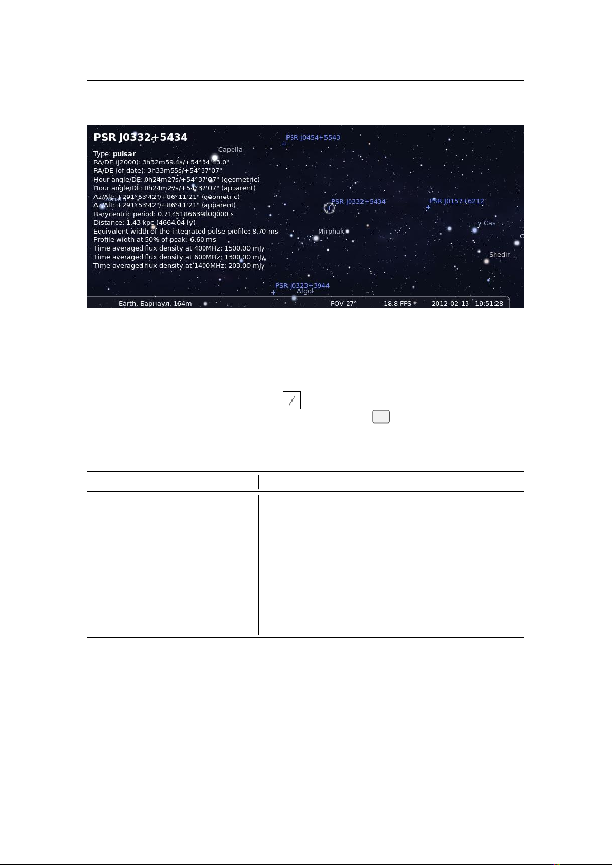
186 Chapter 14. Object Catalog Plugins
Faso. Its source is in the heart of the Sahara Burkinabe and ends in Ghana.
Nikawiy (HD 136418) – Nikawiy is the word for mother in the Indigenous Cree language of Canada.
Awasis (HD 136418 b) – Awasis is the word for child in the Indigenous Cree language of Canada.
Pincoya
(HD 164604) – Pincoya is a female water spirit from southern Chilean mythology who is said to
bring drowned sailors to the Caleuche so that they can live in the afterlife.
Caleuche
(HD 164604 b) – Caleuche is a large ghost ship from southern Chilean mythology which sails the
seas around the island of Chiloé at night.
Lionrock
(HD 212771) – Lion Rock is a lion-shaped peak overlooking Hong Kong and is a cultural symbol
with deep respect from the local community.
Victoriapeak
(HD 212771 b) – Victoria Peak overlooks the bustling Victoria Harbour and is regarded as an
ambassadorial gateway for foreign visitors wishing to experience Hong Kong first hand.
Xihe
(HD 173416) – Xiheis the goddess of the sun in the Chinese mythology and also represents the earliest
astronomers and developers of calendars in ancient China.
Wangshu
(HD 173416 b) – Wangshu is the goddess who drives for the Moon and also represents the Moon
in Chinese mythology.
Formosa
(HD 100655) – Formosa is the historical name of Taiwan used in the
17
th
century, meaning
beautiful in Latin.
Sazum
(HD 100655 b) – Sazum is the traditional name of Yuchi, a Township in Nantou county, in which
the famous Sun-Moon Lake lies. Sazum means water in the language of the Thao people who are a
tribe of Taiwanese aborigines who lived in the region for hundreds of years.
Macondo
(HD 93083) – Macondo is the mythical village of the novel “One Hundred Years of Solitude”
(“Cien años de soledad”) the classic novel by Gabriel García Marquez. Macondo is a fictional place
where magic and reality are mixed.
Melquíades
(HD 93083 b) – Melquíades is a fictional character that walks around Macondo, like a planet
orbiting a star, connecting it with the external world by introducing new knowledge using his inventions
as well as his stories.
Poerava
(HD 221287) – Poerava is the word in the Cook Islands Maori language for a large mystical black
pearl of utter beauty and perfection.
Pipitea
(HD 221287 b) – Pipitea is a small, white and gold pearl found in Penrhyn lagoon in the northern
group of the Cook Islands.
Dìwö
(WASP-17) – Dìwö in Bribri language means the sun (bigger than the sun we know) and that never
turns off.
Ditsö (WASP-17 b) – Ditsö is the name that the god Sibö gave to the first Bribri people.
Stribor
(HD 75898) – Stribor is God of winds in Slavic mythology, as well as a literature character in the
book Pri
ˇ
ce iz davnine (Croatian Tales of Long Ago) by the Croatian author Ivana Brli
´
c-Mažurani
´
c.
Veles (HD 75898 b) – Veles is a major Slavic god of earth, waters and the underworld.
Felixvarela
(BD-17 63) – Felix Varela (1788–1853) was the first to teach science in Cuba at the San Carlos
and San Ambrosio Seminary. He opened the way to education for all, and began the experimental
teaching of physics in Cuba.
Finlay
(BD-17 63 b) – Carlos Juan Finlay (1833–1915) was an epidemiologist recognized as a pioneer in
the research of yellow fever, determining that it was transmitted through mosquitoes.
Alasia
(HD 168746) – Alasia is the first historically recorded name of Cyprus, dating back to mid-fifteenth
century BC.
Onasilos
(HD 168746 b) – Onasilos is the oldest historically recorded doctor in Cyprus, inscribed on the
fifth century BC Idalion Tablet. Also known as the Onasilou Plate, it is considered as the oldest legal
contract found in the world.
Absolutno
(XO-5) – Absolutno is a fictional miraculous substance in the sci-fi novel “Továrna na absolutno”
(“The Factory for the Absolute”) by influential Czech writer Karel
ˇ
Capek.
Makropulos
(XO-5 b) – Makropulos is the name from Karel
ˇ
Capek’s play V
ˇ
ec Makropulos (The Makropu-
los Affair), dealing with problems of immortality and consequences of an artificial prolongation of
life.
Muspelheim
(HAT-P-29) – Muspelheim is the Norse mythological realm of fire. The first gods used the
sparks of Muspelheim to form the sun, moon, planets, and stars.
Surt
(HAT-P-29 b) – Surt is the ruler of Muspelheim and the fire giants there in Norse mythology. At
Ragnarok, the end of the world, he will lead the attack on our world and destroy it in flames.
Márohu
(WASP-6) – Márohu the god of drought is the protector of the Sun and is engraved at a higher
position on the stalagmite than Boinayel in the El Puente cave, where the Sun makes its way down

14.3 Exoplanets Plugin 187
every 21 December.
Boinayel
(WASP-6 b) – Boinayel the god of rain that fertilizes the soil is engraved on the stalagmite at a
lower position than Márohu in the El Puente cave.
Nenque
(HD 6434) – Nenque means the Sun in the language spoken by the Indigenous Waorani tribes of
the Amazon regions of Ecuador
Eyeke
(HD 6434 b) – Eyeke means near in the language spoken by the Indigenous Waorani tribes of the
Amazon regions of Ecuador. This word is suggested for the exoplanet owing to the proximity of the
planet to the host star.
Citalá (HD 52265) – Citalá means River of stars in the native Nahuat language.
Cayahuanca
(HD 52265 b) – Cayahuanca means The rock looking at the stars in the native Nahuat language.
Koit (XO-4) – Koit is Estonian for the time when the Sun rises in the morning (dawn).
Hämarik (XO-4 b) – Hämarik is Estonian for the time when the Sun goes down in the evening (twilight).
Buna (HD 16175) – Buna is the commonly used word for coffee in Ethiopia.
Abol
(HD 16175 b) – Abol is the first of three rounds of coffee in the Ethiopian traditional coffee ceremony.
Horna (HAT-P-38) – Horna is hell or the underworld from Finnic mythology.
Hiisi (HAT-P-38 b) – Hiisi represents sacred localities and later evil spirits from Finnic mythology.
Bélénos (HD 8574) – Bélénos was the god of light, of the Sun, and of health in Gaulish mythology.
Bélisama
(HD 8574 b) – Bélisama was the goddess of fire, notably of the hearth and of metallurgy and
glasswork, in Gaulish mythology.
Itonda (HD 208487) – Itonda, in the Myene tongue, corresponds to all that is beautiful.
Mintome
(HD 208487 b) – Mintome, in the Fang tongue, is a mythical land where a brotherhood of brave
men live.
Mago
(HD 32518) – Mago is a National Park in Ethiopia noted for its giraffes. The star also happens to be
in the constellation of Camelopardis (the giraffe).
Neri (HD 32518 b) – The Neri river in Ethiopia runs through parts of the Mago National park.
Sika (HD 181720) – Sika means gold in the Ewe language and gold is one of Ghana’s principal exports.
Toge (HD 181720 b) – Toge means earring in the Ewe language.
Lerna (HAT-P-42) – Lerna was the name of a lake in the eastern Peloponnese, where the Lernaean Hydra,
an immortal mythical nine-headed beast lived. The star lies in the constellation of Hydra.
Iolaus
(HAT-P-42 b) – Iolaus was the nephew of Heracles from Greek mythology, moving around lake Lerna
in helping Heracles to exterminate the Lernaean Hydra. Similarly this exoplanet in the constellation
of Hydra moves around its parent star.
Tojil (WASP-22) – Tojil is the name of one of the Mayan deities related to rain, storms, and fire.
Koyopa’
(WASP-22 b) – Koyopa’ is the word associated with lightning in K’iche’ (Quiché) Mayan language.
Citadelle
(HD 1502) – The Citadelle is a large mountaintop fortress in Nord, Haiti built after Haiti’s
independence, and was designated a UNESCO World Heritage site along with the nearby Sans-Souci
Palace.
Indépendance
(HD 1502 b) – Indépendance is named after the Haitian Declaration of Independence on 1
January 1804, when Haiti became the first independent black republic.
Hunahpú
(HD 98219) – Hunahpú was one of the twin gods who became the Sun in K’iche’ (Quiché)
Mayan mythology as recounted in the Popol Vuh.
Ixbalanqué
(HD 98219 b) – Ixbalanqué was one of the twin gods who became the Moon in K’iche’ (Quiché)
Mayan mythology as recounted in the Popol Vuh.
Hunor
(HAT-P-2) – Hunor was a legendary ancestor of the Huns and the Hungarian nation, and brother of
Magor.
Magor
(HAT-P-2 b) – Magor was a legendary ancestor of the Magyar people and the Hungarian nation, and
brother of Hunor.
Funi (HD 109246) – Funi is an old Icelandic word meaning fire or blaze.
Fold (HD 109246 b) – Fold is an old Icelandic word meaning earth or soil.
Bibh
¯
a
(HD 86081) – Bibh
¯
a is the Bengali pronunciation of the Sanskrit word Vibha, which means a bright
beam of light.
Santamasa
(HD 86081 b) – Santamasa in Sanskrit means clouded, which alludes to the exoplanet’s
atmosphere.
Dofida (HD 117618) – Dofida means our star in Nias language.
Noifasui
(HD 117618 b) – Noifasui means revolve around in Nias language, derived from the word ifasui,
meaning to revolve around, and no, indicating that the action occurred in the past and continued to the
present time.
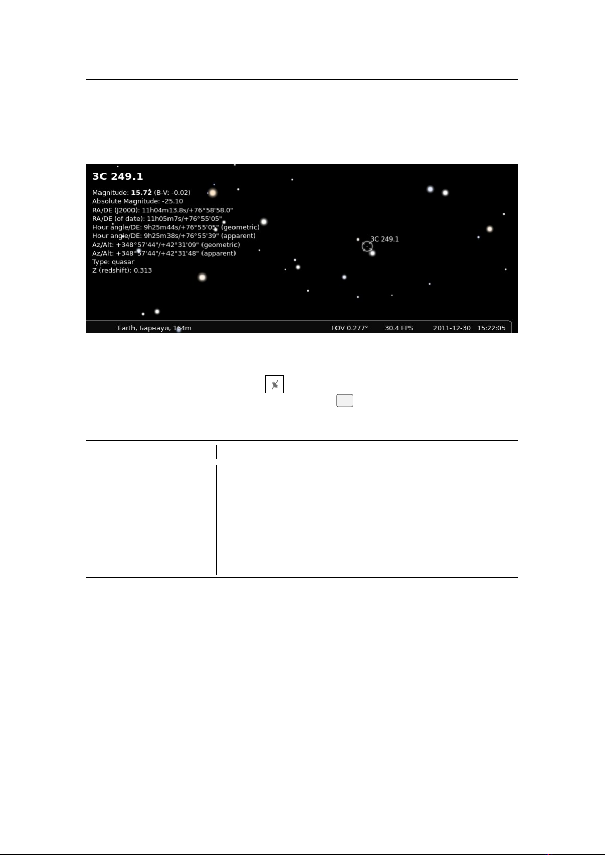
188 Chapter 14. Object Catalog Plugins
Kaveh
(HD 175541) – Kaveh is one of the heroes of Shahnameh, the epic poem composed by Persian poet
Ferdowsi between 977 and 1010 CE. Kaveh is a blacksmith who symbolises justice.
Kavian
(HD 175541 b) – Kaveh carries a banner called Derafsh Kaviani (Derafsh: banner, Kaviani: relating
to Kaveh).
Uruk
(HD 231701) – Uruk was an ancient city of the Sumer and Babylonian civilizations in Mesopotamia
situated along an ancient channel of the Euphrates river in modern-day Iraq.
Babylonia
(HD 231701 b) – Babylonia was a key kingdom in ancient Mesopotamia from the
18
th
to
6
th
centuries BC whose name-giving capital city was built on the Euphrates river.
Tuiren
(HAT-P-36) – Tuiren was the aunt of the hunterwarrior Fionn mac Cumhaill of Irish legend, who
was turned into a hound by the jealous fairy Uchtdealbh.
Bran
(HAT-P-36 b) – Tuiren’s son Bran was a hound and cousin of the hunterwarrior Fionn mac Cumhaill
of Irish legend.
Tevel
(HAT-P-9) – Tevel means Universe or everything and begins with the letter Taf, the last letter in the
Hebrew alphabet.
Alef (HAT-P-9 b) – Alef is the first letter in the Hebrew alphabet and also means bull.
Flegetonte
(HD 102195) – Flegetonte is the underworld river of fire from Greek Mythology in the Italian
narrative poem on the afterlife “Divina Commedia” (“Divine Commedy”) by Dante Alighieri, chosen
as an allusion to the star’s fiery nature.
Lete
(HD 102195 b) – Lete is the oblivion river made of fog from Greek Mythology in the Italian narrative
poem on the afterlife “Divina Commedia” (“Divine Commedy”) by Dante Alighieri, chosen as an
allusion to the planet’s gaseous nature.
Nyamien (WASP-15) – Nyamien refers to the supreme creator deity of Akan mythology.
Asye (WASP-15 b) – Asye refers to the Earth goddess of Akan mythology.
Kamui
(HD 145457) – Kamui is a word in the Ainu language denoting a supernatural entity possessing
spiritual energy.
Chura (HD 145457 b) – Chura is a word in the Ryukyuan/Okinawan language meaning natural beauty.
Petra
(WASP-80) – Petra is a historical and archaeological city in southern Jordan and a UNESCO World
Heritage site.
Wadirum
(WASP-80 b) – Wadi Rum (Valley of the Moon) is located at the far south of Jordan, it is the
largest valley in Jordan, set on the high plateau at the western edge of the Arabian Desert.
Kalausi
(HD 83443) – The word Kalausi means a very strong whirling column of wind in the Dholuo
language of Kenya.
Buru
(HD 83443 b) – Buru means dust in the Dholuo language of Kenya and is typically associated with
wind storms.
Liesma
(HD 118203) – Liesma means flame, and it is the name of a character from the Latvian poem
Staburags un Liesma.
Staburags
(HD 118203 b) – Staburags is the name of a character from the Latvian poem Staburags un
Liesma, and denotes a rock with symbolic meaning in literature and history.
Phoenicia
(HD 192263) – Phoenicia was an ancient thalassocratic civilisation of the Mediterranean that
originated from the area of modern-day Lebanon.
Beirut
(HD 192263 b) – Beirut is one of the oldest continuously inhabited cities in the world and was a
Phoenician port. Beirut is now the capital and largest city of Lebanon.
Pipoltr
(TrES-3) – In the local dialect of Triesenberg, Pipoltr is a bright and visible butterfly, alluding to the
properties of a star.
Umbäässa
(TrES-3 b) – In the local dialect of southern Liechtenstein, Umbäässa is a small and barely
visible ant, alluding to the properties of a planet with respect to its star.
Taika (HAT-P-40) – Taika means peace in the Lithuanian language.
Vytis (HAT-P-40 b) – Vytis is the symbol of the Lithuanian coat of arms.
Lucilinburhuc
(HD 45350) – The Lucilinburhuc fortress was built in 963 by the founder of Luxembourg,
Count Siegfried.
Peitruss
(HD 45350 b) – Peitruss is derived from the name of the Luxembourg river Pétrusse, with the
river’s bend around Lucilinburhuc fortress alluding to the orbit of the planet around its star.
Rapeto (HD 153950) – Rapeto is a giant creature from Malagasy tales.
Trimobe (HD 153950 b) – Trimobe is a rich ogre from Malagasy tales.
Intan
(HD 20868) – Intan means diamond in the Malay language (Bahasa Melayu), alluding to the shining
of a star.
Baiduri
(HD 20868 b) – Baiduri means opal in Malay language (Bahasa Melayu), alluding to the mysterious

14.3 Exoplanets Plugin 189
beauty of the planet.
Sansuna
(HAT-P-34) – Sansuna is the name of the mythological giant from traditional Maltese folk tales
that carried the stones of the Gozo megalithic temples on her head.
˙
Ggantija
(HAT-P-34 b) –
˙
Ggantija means giantess: the megalithic temple complex on the island of Gozo,
which alludes to the grandeur of this gas giant exoplanet.
Diya
(WASP-72) – Diya is an oil lamp that is brought by Indian ancestors to Mauritius in the 1820’s, and is
used for lighting during special occasions, including the light festival of Diwali.
Cuptor
(WASP-72 b) – Cuptor is a thermally insulated chamber used for baking or drying substances, that
has long disappeared in Mauritius and has been replaced by more sophisticated ovens.
Axólotl
(HD 224693) – Axólotl means water animal in the native Nahuatl language, which is a unique and
culturally significant endemic amphibious species from the basin of Mexico.
Xólotl
(HD 224693 b) – Xólotl means animal in the native Nahuatl language and was an Aztec deity
associated with the evening star (Venus).
Tislit
(WASP-161) – Tislit is the name of a lake in the Atlas mountains of Morocco. It means the bride in
the Amazigh language and it is associated with a heartbroken beautiful girl in an ancient local legend.
Isli
(WASP-161 b) – Isli is the name of a lake in the Atlas mountains of Morocco. It means the groom in the
Amazigh language and it is associated with a heartbroken handsome boy in an ancient local legend.
Emiw
(HD 7199) – Emiw represents love in the local Makhuwa language of the northern region of
Mozambique.
Hairu
(HD 7199 b) – Hairu represents unity in the local Makhuwa language of the northern region of
Mozambique.
Ayeyarwady (HD 18742) – Ayeyarwady is the largest and most important river in Myanmar.
Bagan (HD 18742 b) – Bagan is one of Myanmar’s ancient cities that lies beside the Ayeyarwardy river.
Sagarmatha
(HD 100777) – Sagarmatha is the Nepali name for the highest peak in the world (also known
as Mount Everest) and symbol of national pride of Nepal.
Laligurans
(HD 100777 b) – Laligurans are the Nepali variation of the rhododendron flower and is the
national flower of Nepal.
Sterrennacht
(HAT-P-6) – The Sterrennacht (Starry Night) is a world-famous painting by Dutch grand
master Van Gogh that was painted in France in 1889 and now belongs to the permanent collection of
New York’s Museum of Modern Art.
Nachtwacht
(HAT-P-6 b) – The Nachtwacht (Night Watch) is a world-famous painting by Dutch grand
master Rembrandt that was completed in 1642 and now belongs to the collection of the Rijksmuseum
in Amsterdam.
Karaka
(HD 137388) – Karaka is the word in the M
¯
aori language for a plant endemic to New Zealand that
produces a bright orange, fleshy fruit.
Kerer
¯
u
(HD 137388 b) – Kerer
¯
u is the word in the M
¯
aori language for a large bush pigeon native to New
Zealand.
Cocibolca
(HD 4208) – Cocibolca is the Nahualt name for the largest lake in Central America in Nicaragua.
Xolotlan
(HD 4208 b) – Xolotlan is the name of the second largest lake of Nicaragua and its name is from
the Nahualt language of the indigenous tribe that settled in Nicaragua, which symbolises a native god
and a refuge for animals.
Amadioha
(HD 43197) – Amadioha is the god of thunder in Igbo mythology. As well as representing
justice, Amadioha is also a god of love, peace and unity.
Equiano
(HD 43197 b) – Equiano was a writer and abolitionist from Ihiala, Nigeria who fought injustice
and the elimination of the slave trade.
Násti (HD 68988) – Násti means star in the Northern Sami language of Norway.
Albmi (HD 68988 b) – Albmi means sky in the Northern Sami language of Norway.
Shama
(HAT-P-23) – Shama is an Urdu literary term meaning a small lamp or flame, symbolic of the light
of the star.
Perwana
(HAT-P-23 b) – Perwana means moth in Urdu, alluding to the eternal love of an object circling the
source of light (the lamp).
Moriah (HD 99109) – Moriah is an ancient name for the mountain within the Old City of Jerusalem.
Jebus
(HD 99109 b) – Jebus was the ancient name of Jerusalem in
2
nd
millennium BC when populated by
the Canaanite tribe of Jebusites.
Montuno
(WASP-79) – Montuno is the traditional costume the man wears in the “El Punto”, a Panamanian
dance in which a man and woman dance to the sound of drums.
Pollera
(WASP-79 b) – Pollera is the traditional costume the woman wears in the El Punto, a Panamanian
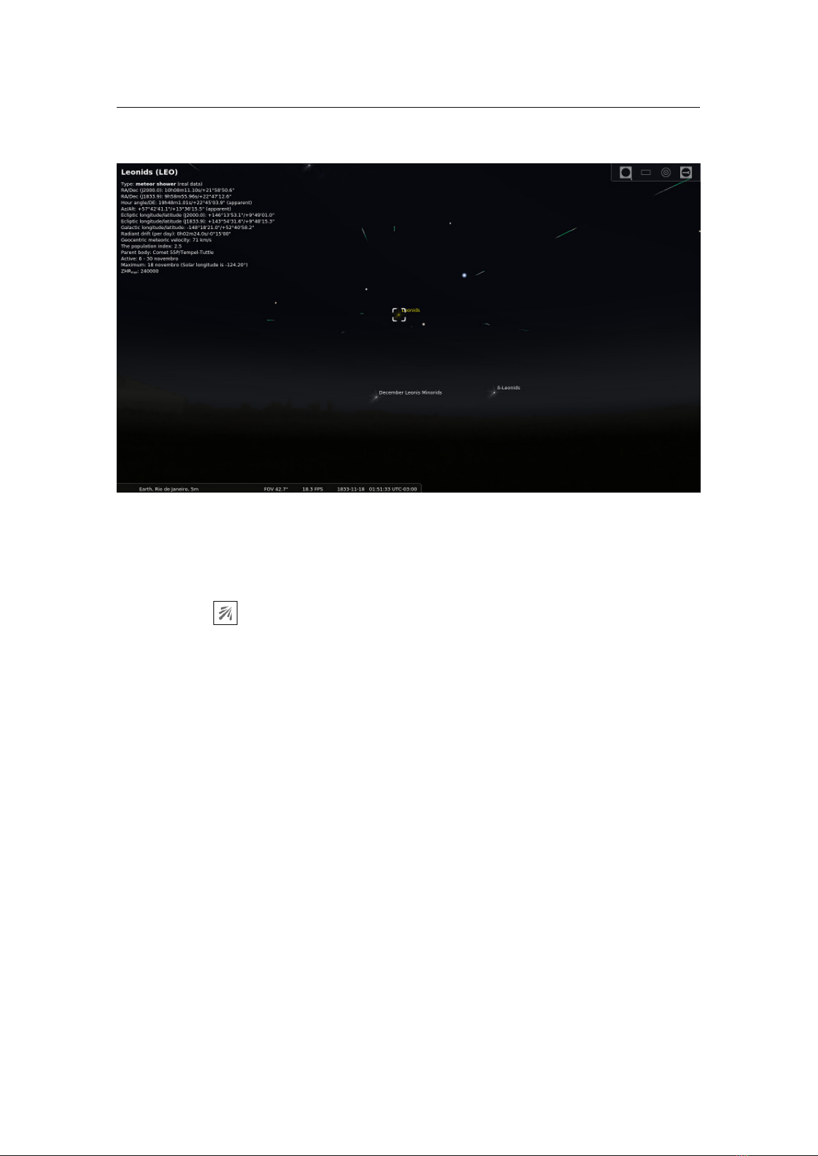
190 Chapter 14. Object Catalog Plugins
dance in which a man and woman dance to the sound of drums.
Tupã
(HD 108147) – Tupã is one of four principle gods of the Guarani Cosmogony in popular Paraguayan
folklore that helped the supreme god Ñamandu to create the Universe.
Tumearandu
(HD 108147 b) – Tume Arandu is a son of Rupavê and Sypavê, the original man and woman
of the Universe, who is known as the Father of Wisdom in popular Paraguayan folklore.
Inquill
(HD 156411) – Inquil was one half of the couple involved in the tragic love story Way to the Sun by
famous Peruvian writer Abraham Valdelomar.
Sumajmajta
(HD 156411 b) – Sumaj Majta was one half of the couple involved in a tragic love story Way
to the Sun by famous Peruvian writer Abraham Valdelomar.
Amansinaya
(WASP-34) – Aman Sinaya is one of the two trinity deities of the Philippine’s Tagalog
mythology, and is the primordial deity of the ocean and protector of fisherman.
Haik
(WASP-34 b) – Haik is the successor of the primordial Aman Sinaya as the God of the Sea of the
Philippine’s Tagalog mythology.
Uklun (HD 102117) – Uklun means us or we in the Pitkern language of the people of Pitcairn Islands.
Leklsullun
(HD 102117 b) – Lekl Sullun means child or children in the Pitkern language of the people of
Pitcairn Islands.
Solaris
(BD+14 4559) – Solaris is the title of a 1961 science fiction novel about an ocean-covered exoplanet
by Polish writer Stanislaw Lem.
Pirx
(BD+14 4559 b) – Pirx is a fictional character from books by Polish science-fiction writer Stanislaw
Lem.
Lusitânia
(HD 45652) – Lusitânia is the ancient name of the western region of the Iberic Peninsula where
the Lusitanian people lived and where most of modern-day Portugal is situated.
Viriato
(HD 45652 b) – Viriato was a legendary leader of the Lusitanian people, a herdsman and hunter
who led the resistance against Roman invaders during 2
nd
century B.C.
Koeia
(HIP 12961) – Koeia was the word for star in the language of the Taíno Indigenous People of the
Caribbean.
Aumatex
(HIP 12961 b) – Aumatex was the God of Wind in the mythology of the Taíno Indigenous People
of the Caribbean.
Moldoveanu
(XO-1) – Moldoveanu is the highest peak in Romania of the F
˘
ag
˘
ara
s
,
mountain range with an
altitude of 2544 metres.
Negoiu
(XO-1 b) – Negoiu is the second highest peak in Romania of the F
˘
ag
˘
ara
s
,
mountain range with an
altitude of 2535 metres.
Dombay
(HAT-P-3) – Dombay is a resort region in the North Caucasus mountains that is enclosed by
mountain forests and rich wildlife, including bears (as this star lies in the constellation Ursa Major,
the great bear).
Teberda
(HAT-P-3 b) – Teberda is a mountain river in Dombay region with a rapid water flow, symbolising
the planet’s rapid motion around its host star.
Belel (HD 181342) – Belel is a rare source of water in the north of Senegal.
Dopere
(HD 181342 b) – Dopere is an expansive historical area in the north of Senegal where Belel was
located.
Morava (WASP-60) – Morava is the longest river system in Serbia.
Vlasina (WASP-60 b) – Vlasina is one of the most significant tributaries of the South Morava river.
Parumleo
(WASP-32) – Parumleo is a Latin term for little lion, symbolising Singapore’s struggle for
independence.
Viculus
(WASP-32 b) – Viculus is a Latin term for little village, embodying the spirit of the Singaporean
people.
Chaso
ˇ
n (HAT-P-5) – Chaso
ˇ
n is an ancient Slovak term for Sun.
Král’omoc (HAT-P-5 b) – Král’omoc is an ancient Slovak term for the planet Jupiter.
Irena
(WASP-38) – Irena is a leading character in the novel “Under the Free Sun: a Story of the Ancient
Grandfathers” by Slovene writer Fran Saleški Finžgar. Irena is a woman of the court.
Iztok
(WASP-38 b) – Iztok is a leading character in the novel “Under the Free Sun: a Story of the Ancient
Grandfathers” by Slovene writer Fran Saleški Finžgar. Iztok is a freedom fighter for the Slavic people.
Naledi
(WASP-62) – Naledi means star in the Sesotho, SeTswana and SePedi languages and is typically
given as a name to girls in the hope that they will bring light, joy and peace to their communities.
Krotoa
(WASP-62 b) – Krotoa is considered the Mother of Africa and member of the indigenous Khoi
people, who was a community builder and educator during colonial times.
Baekdu
(8 Umi) – Baekdu is the highest mountain on the Korean peninsula, situated in North Korea, and
14.3 Exoplanets Plugin 191
symbolises the national spirit of Korea.
Halla
(8 Umi b) – Halla is the highest mountain in South Korea and is regarded as a sacred place in the
region.
Rosalíadecastro
(HD 149143) – Rosalía de Castro was a significant figure of Galician culture and prominent
Spanish writer, whose pioneeting work often referenced the night and celestial objects.
Riosar
(HD 149143 b) – Rio Sar is the name of a river that was present in much of the literary work of the
pioneering Spanish author Rosalía de Castro.
S
¯
amaya (HD 205739) – S
¯
amaya means peace in the Sinhalese language.
Samagiya (HD 205739 b) – Samagiya means togetherness and unity in the Sinhalese language.
Aniara
(HD 102956) – Aniara is the name of a spaceship in the epic poem Aniara by Swedish author Harry
Martinson.
Isagel
(HD 102956 b) – Isagel is the name of the spaceship pilot in the epic science fiction poem Aniara
written by Swedish author Harry Martinson.
Mönch (HD 130322) – Mönch is one of the prominent peaks of the Bernese Alps in Switzerland.
Eiger
(HD 130322 b) – Eiger is one of the prominent peaks of the Bernese Alps, in the Jungfrau-Aletsch
protected area.
Ebla
(HD 218566) – Ebla was one of the earliest kingdoms in Syria, and served as a prominent region in
the 2
nd
and 3
rd
millennia B.C.
Ugarit
(HD 218566 b) – Ugarit was a city where its scribes devised the Ugaritic alphabet around 1400 B.C.
The alphabet was made up of thirty letters and was inscribed on clay tablets.
Mpingo
(WASP-71) – Mpingo is a famous tree that grows in southern Tanzania and produces ebony wood
used for musical instruments and curios.
Tanzanite
(WASP-71 b) – Tanzanite is the name of a precious stone mined in Tanzania and is treasured
worldwide.
Chaophraya (WASP-50) – Chao Phraya is the great river of Thailand.
Maeping (WASP-50 b) – Mae Ping is one of the tributaries of Thailand’s great river Chao Phraya.
Atakoraka (WASP-64) – Atakoraka means the chain of the Atacora: the largest mountain range in Togo.
Agouto
(WASP-64 b) – Agouto (Mount Agou) is the highest mountain in Togo and a treasured region of
the Atakoraka.
Dingolay
(HD 96063) – Dingolay means to dance, twist and turn in elaborate movements, symbolising the
culture and language of the ancestors of the people of Trinidad and Tobago.
Ramajay
(HD 96063 b) – Ramajay means to sing and make music in a steelpan style, representing the love
of culture and languages of the ancestors of the people of Trinidad and Tobago.
Chechia
(HD 192699) – Chechia is a flat-surfaced, traditional red wool hat worn by men and women,
symbolising the country’s rich traditions and is considered as the national headdress for in Tunisia.
Khomsa
(HD 192699 b) – Khomsa is a palm-shaped amulet that is popular in Tunisia, used in jewelry and
decorations. It depicts an open right hand and is often found in modern designs.
Anadolu
(WASP-52) – Anadolu is the primary homeland of Turkey and refers to the motherland in Turkish
culture.
Göktürk
(WASP-52 b) – Göktürk refers to the historical origin of the Turkish people, as it was the first
established state in Turkey in
5
th
century AD. It is also the name of a Turkish satellite and is the
combination of two words, of which “Gök” means sky.
Berehinya
(HAT-P-15) – Berehinya was a Slavic deity of waters and riverbanks but in more recent times
her status has been promoted to that of a national goddess — “hearth mother, protectress of the earth”.
Tryzub
(HAT-P-15 b) – Tryzub is the most recognised ancient symbol of Ukraine, that was minted on the
coins of Prince Volodymyr the Great and today remains one of the country’s state symbols (a small
coat).
Sharjah
(HIP 79431) – Sharjah is the cultural capital of United Arab Emirates, and considered the city of
knowledge due to its many educational centers, institutes, museums, libraries and heritage centers.
Barajeel
(HIP 79431 b) – A barajeel is a wind tower used to direct the flow of the wind so that air can be
recirculated as a form of air conditioning.
Gloas (WASP-13) – In Manx Gaelic, Gloas means to shine (like a star).
Cruinlagh (WASP-13 b) – In Manx Gaelic, Cruinlagh means to orbit (like a planet around its star).
Nushagak
(HD 17156) – Nushagak is a regional river near Dilingham, Alaska, which is famous for its wild
salmon that sustain local Indigenous communities.
Mulchatna
(HD 17156 b) – The Mulchatna River is a tributary of the Nushagak River in southwestern
Alaska, USA.

192 Chapter 14. Object Catalog Plugins
Ceibo (HD 63454) – Ceibo is the name of the native tree of Uruguay that gives rise to the national flower.
Ibirapitá
(HD 63454 b) – Ibirapitá is the name of a native tree that is characteristic of the country of
Uruguay, and is also known as Artigas’ tree, after the national hero.
Natasha (HD 85390) – Natasha means thank you in many languages of Zambia.
Madalitso (HD 85390 b) – Madalitso means blessings in the native language of Nyanja in Zambia.
All names with asterix mark (*) are modified based on the original proposals, to be consistent with the
IAU rules.
14.3.3 Section
[
Exoplanets
]
in config.ini file
You can edit config.ini file to change the settings for the Exoplanets plugin – just make it carefully!
ID Type Description
last_update string Date and time of last update
update_frequency_hours
int Frequency of updates, in hours
updates_enable
bool Enable updates of exoplanets catalog from Internet
url
string URL of exoplanets catalog
flag_show_exoplanets_button
bool Enable showing button of exoplanets on bottom bar
distribution_enabled
bool Enable distribution mode of display
timeline_enabled
bool Enable timeline mode of display
habitable_enabled
bool Enable habitable mode of display
enable_at_startup
bool Enable displaying exoplanets at startup of the plugin
exoplanet_marker_color
R,G,B Color for marker of star with planetary system
habitable_exoplanet_marker_color
R,G,B
Color for marker of star with planetary system with
potential habitable exoplanets
temperature_scale
string
Temperature scale for equilibrium temperature of exo-
planets. Possible values: Kelvin, Celsius, Fahrenheit.
Default value: Celsius.
14.3.4 Format of exoplanets catalog
To add a new exoplanet system, open a new line after line 5 and paste the following, note commas and
brackets, they are important:
" Star de sig na t io n ":
{
" exo pla net s ":
[
{
" mass ": mass of ex opl ane t ( M jup ) ,
" radius " : radius of exop lane t ( R jup ),
" period " : period of exop lane t ( days ),
" semiA xis " : semi - major axis ( AU) ,
" ecc en tri ci ty " : orbit ’s eccentrici ty ,
" inc lin at ion ": orbit ’s i nc lin at ion ( d egree ) ,
" ang le Di st a nc e ": angle distan ce from star ( arc sec ond s ),
" dis cov ere d ": exopl ane t d isc ove red year ,
" de te cti on Me th od ": " e xop lane t d ete c tio n metho d ",
" pclass " : " p lane tar y class " ,
" EqTemp " : e qui lib ri um t em per atu re ( K),
" con se rva ti ve " : cons erv at ive or opt imi sti c
hab ita bi lit y of the exoplanet ,
" ESI ": Earth Simi la rit y Index (*100) ,
" pl an et Pr op er Na me " : " pr oper name of pla net " ,
" pla net Nam e ": " des ig nat ion of planet "
},
{
" mass ": mass of ex opl ane t ( M jup ) ,
" radius " : radius of exop lane t ( R jup ),
" period " : period of exop lane t ( days ),
" semiA xis " : semi - major axis ( AU) ,

14.3 Exoplanets Plugin 193
" ecc en tri ci ty " : orbit ’s eccentrici ty ,
" inc lin at ion ": orbit ’s i nc lin at ion ( d egree ) ,
" ang le Di st a nc e ": angle distan ce from star ( arc sec ond s ),
" dis cov ere d ": exopl ane t d isc ove red year ,
" de te cti on Me th od ": " e xop lane t d ete c tio n metho d ",
" pclass " : " p lane tar y class " ,
" EqTemp " : e qui lib ri um t em per atu re ( K),
" con se rva ti ve " : cons erv at ive or opt imi sti c h ab ita bi li t y of the
exoplanet ,
" ESI ": Earth Simi la rit y Index (*100) ,
" pl an et Pr op er Na me " : " pr oper name of pla net " ,
" pla net Nam e ": " des ig nat ion of planet "
}
],
" dista nce " : value of distan c e to star ( pc ),
" stype ": " sp ectr al type of star " ,
" smass ": value of mass of star (M sun ),
" smetal " : value of metal li cit y of star ,
" Vmag ": value of v isual ma gni tude of star ,
" sradius ": value of radi u s of star (R sun ),
" eff ec ti ve T em p ": value of eff ecti ve t em per atu re of star (K ),
" st arP ro pe rN am e ": " proper name of the star " ,
" hasHP ": boole an ( has pot enti al h abi tabl e pl anets ) ,
" RA ": " Right asc ens ion ( J2000 ) ",
" DE ": " Decli na tio n ( J2000 ) "
},
For example, the record for 24 Sex looks like:
" 24 Sex ":
{
" exo pla net s ":
[
{
" mass ": 1.99 ,
" period " : 452.8 ,
" semiA xis " : 1.333 ,
" ecc en tri ci ty " : 0.09 ,
" ang le Di st a nc e ": 0.017821 ,
" dis cov ere d ": 2010 ,
" pla net Nam e ": "b "
},
{
" mass ": 0.86 ,
" period " : 883.0 ,
" semiA xis " : 2.08 ,
" ecc en tri ci ty " : 0.29 ,
" ang le Di st a nc e ": 0.027807 ,
" dis cov ere d ": 2010 ,
" pla net Nam e ": "c "
}
],
" dista nce " : 74.8 ,
" stype ": " G5 ",
" smass ": 1.54 ,
" smetal " : -0.03 ,
" Vmag ": 7.38 ,
" sradius ": 4.9 ,
" eff ec ti ve T em p ": 5098 ,
" RA ": "10 h2 3m28s " ,
" DE ": " -00 d54 m08s "
},
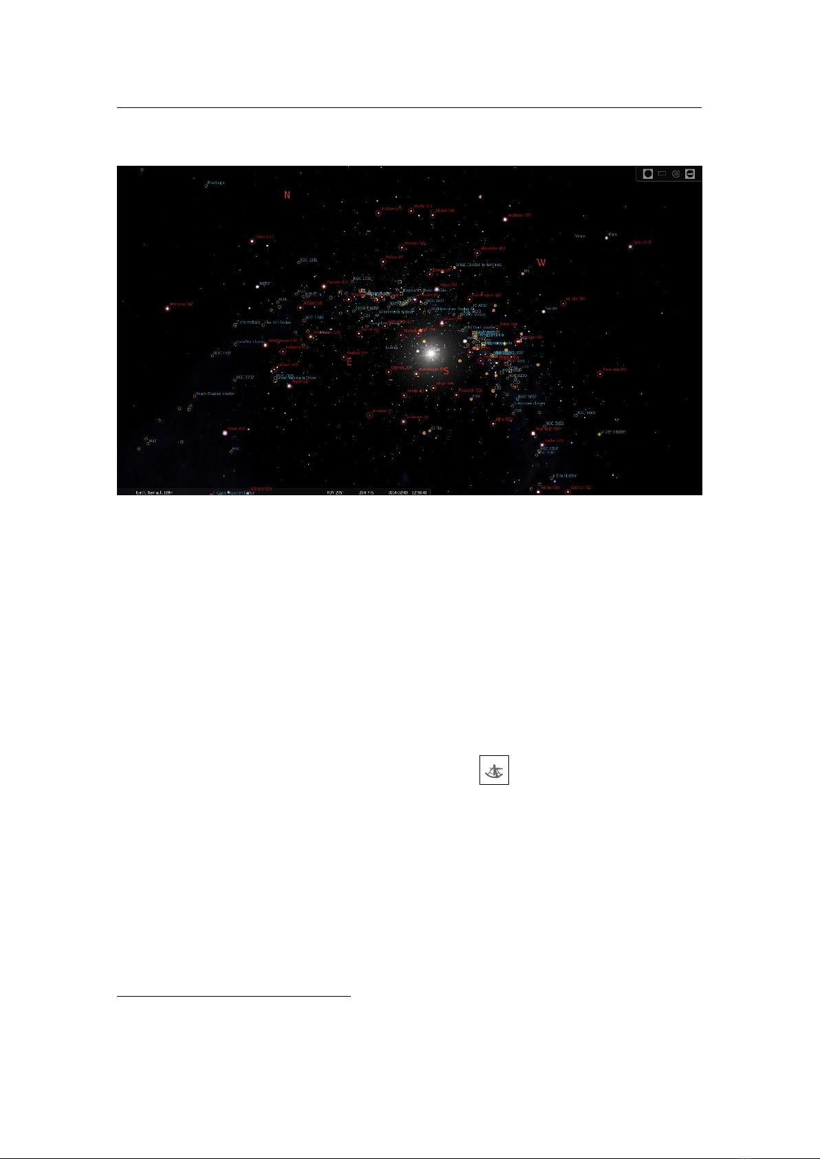
194 Chapter 14. Object Catalog Plugins
14.4 Pulsars Plugin
Figure 14.5: PSR J0332+5434
This plugin plots the position of various pulsars, with object information about each one. Pulsar data is
derived from “The Australia Telescope National Facility Pulsar Catalogue” (Manchester et al., 2005).
If enabled (see section 12.1), use the button to activate display of pulsars. The GUI allows a few
configuration options. You can also find a pulsar (
F3
) by its designation (e.g., PSR J0437-4715).
14.4.1 Section
[
Pulsars
]
in config.ini file
ID Type Description
last_update string Date and time of last update
update_frequency_days
int Frequency of updates [days]
updates_enable
bool Enable updates of pulsars catalog from Internet
url
string URL of pulsars catalog
enable_at_startup
bool Enable displaying of pulsars at startup of Stellarium
distribution_enabled
bool Enable distribution mode for the pulsars
flag_show_pulsars_button
bool Enable displaying pulsars button on toolbar
marker_color
R,G,B Color for marker of the pulsars
glitch_color
R,G,B Color for marker of the pulsars with glitches
use_separate_colors
bool Use separate colors for different types of the pulsars
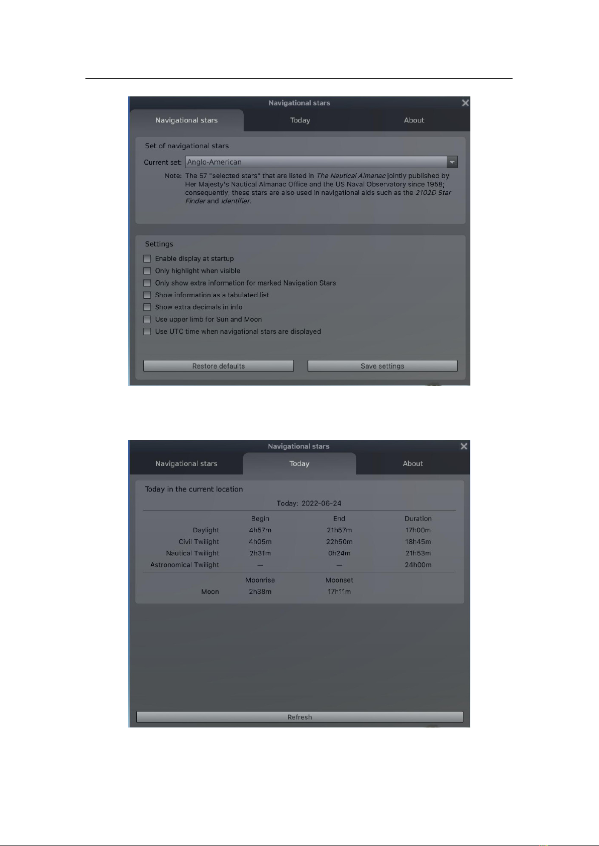
14.4 Pulsars Plugin 195
14.4.2 Format of pulsars catalog
To add a new pulsar, open a new line after line 5 and paste the following, note commas and brackets, they are
important:
" Pulsar de sig nati on ":
{
" RA ": " Right ascensi on ( J2000 )" ,
" DE ": " Declinatio n ( J2000 )" ,
" notes ": " type of pulsar " ,
" distance " : value of d istance based on elec tron density
model ( kpc ) ,
" period ": value of ba ryc entr ic period of the pulsar ( s),
" parallax " : value of annual parallax ( mas ),
" bperiod " : value of binary period of pulsar ( days ) ,
" p der ivat ive ": value of time deri vat ive of barcyce ntri c
period ,
" dmeasure " : value of dispersion measure ( pc /( cm * cm *cm )) ,
" frequency " : value of b ary cent ric rotation fre quency ( Hz ),
" pfre quency ": value of time deri vat ive of barycentric
rota tion fr equency (1/( s *s ))
" e ccen tric ity ": value of eccentricity ,
" w50 ": value of profile width at 50% of peak ( ms ),
" s400 ": value of time averag ed flux d ensity at
400 MHz ( mJy ) ,
" s600 ": value of time averag ed flux d ensity at
600 MHz ( mJy ) ,
" s1400 ": value of time averag ed flux d ensity at
1400 MHz ( mJy )
},
For example, the record for PSR J0014+4746 looks like:
" PSR J0014 +4746 ":
{
" distance " : 1.82 ,
" dmeasure " : 30.85 ,
" frequency " : 0.805997 239145 ,
" pfre quency ": -3.6669 E -16 ,
" w50 ": 88.7 ,
" s400 ": 14 ,
" s600 ": 9 ,
" s1400 ": 3 ,
" RA ": " 00 h14m17 .75 s",
" DE ": " 47 d46m33 .4 s "
},

196 Chapter 14. Object Catalog Plugins
14.5 Quasars Plugin
The Quasars plugin provides visualization of some quasars brighter than 16 visual magnitude. The catalogue
of quasars has been compiled from “A catalogue of quasars and active nuclei: 13th edition” (Véron-Cetty
and Véron, 2010).
Figure 14.6: 3C 249.1, also known as LEDA 2821945 or 4C 77.09
If enabled (see section 12.1), use the button to activate display of quasars. The GUI allows a few
configuration options. You can also find a quasar (
F3
) by its designation (e.g., 3C 273).
14.5.1 Section
[
Quasars
]
in config.ini file
ID Type Description
last_update string Date and time of last update
update_frequency_days
int Frequency of updates, in days
updates_enable
bool Enable updates of quasars catalog from Internet
url
string URL of quasars catalog
enable_at_startup
bool Enable displaying of quasars at startup of Stellarium
distribution_enabled
bool Enable distribution mode for the quasars
flag_show_quasars_button
bool Enable displaying quasars button on toolbar
marker_color
R,G,B Color for marker of the quasars
14.5.2 Format of quasars catalog
To add a new quasar, open a new line after line 5 and create a new section. For example, the record for 3C
249.1 looks like (note commas and brackets – they are important!):
"3C 249.1 ": // Quasar de sign atio n
{
" RA ": " 11 h04m13 .8 s ", // Right ascension ( J2000 )
" DE ": " +76 d58m58s " , // Declina tio n ( J2000 )
" Amag ": -25.1 , // value of absol ute magnitude
" Vmag ": 15.72 , // value of visual ma gni tude
"z": 0.313 , // value of Z ( redshift )
" bV ": -0.02 // value of B -V colour
},
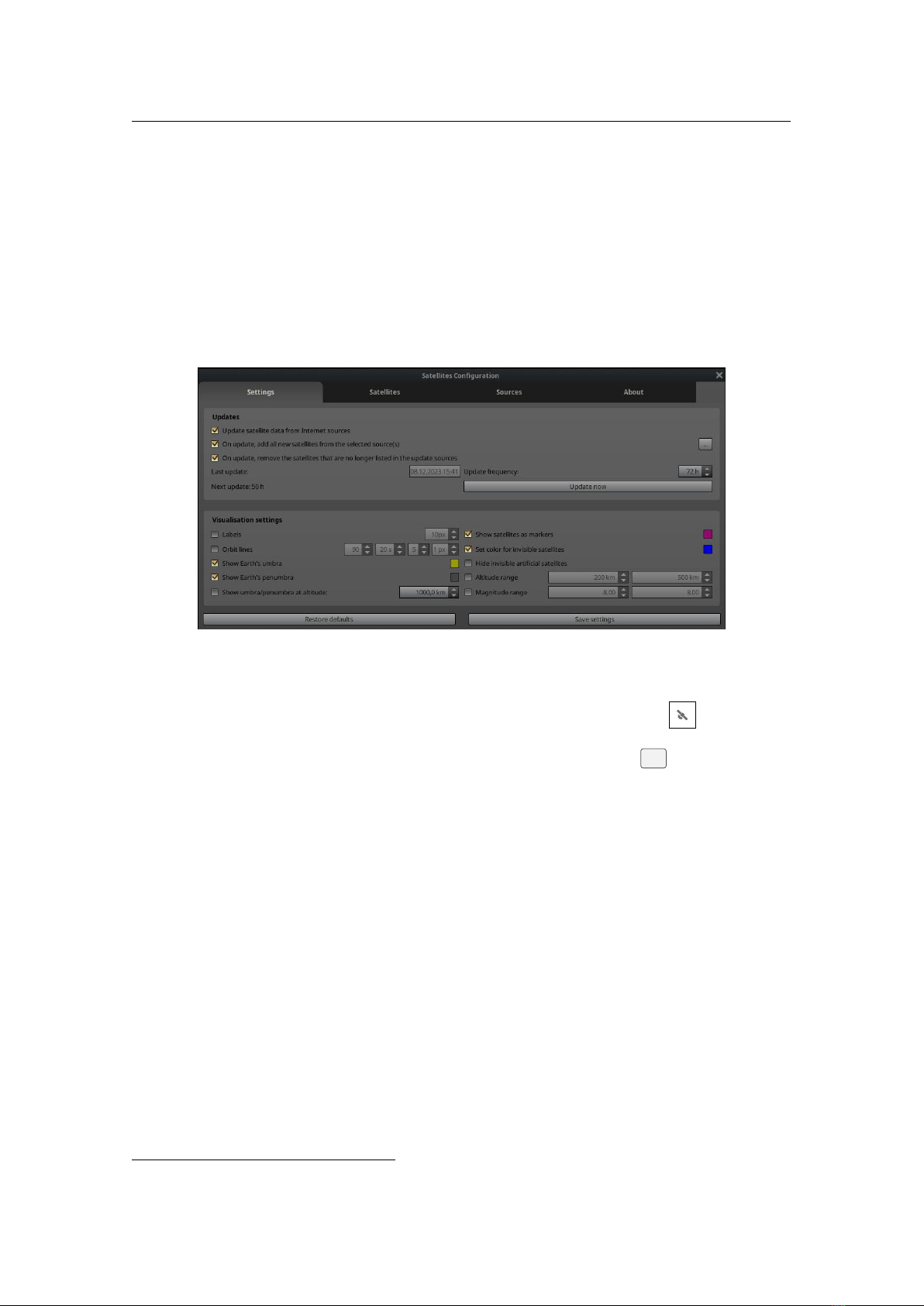
14.6 Meteor Showers Plugin 197
14.6 Meteor Showers Plugin
Figure 14.7: The 1833 Leonids replayed with the Meteor Showers plugin.
In contrast and extension of the random shooting stars feature of Stellarium (see section 19.6), this plugin
provides data for real meteor showers and a marker for each active and inactive radiant, showing real
information about its activity. If enabled (see section 12.1), just click on the Meteor Showers button on
the bottom toolbar to display markers for the radiants.
14.6.1 Terms
Meteor shower
A meteor shower is a celestial event in which a number of meteors are observed to radiate, or originate, from
one point in the night sky. These meteors are caused by streams of cosmic debris called meteoroids entering
Earth’s atmosphere at extremely high speeds on parallel trajectories. Most meteors are smaller than a grain of
sand, so almost all of them disintegrate and never hit the Earth’s surface. Intense or unusual meteor showers
are known as meteor outbursts and meteor storms, which may produce greater than 1,000 meteors an hour.
Radiant
The radiant or apparent radiant of a meteor shower is the point in the sky from which (to a planetary
observer) meteors appear to originate. The Perseids, for example, are meteors which appear to come from a
point within the constellation of Perseus.
An observer might see such a meteor anywhere in the sky but the direction of motion, when traced back,
will point to the radiant. A meteor that does not point back to the known radiant for a given shower is known
as a sporadic and is not considered part of that shower.
Many showers have a radiant point that changes position during the interval when it appears. For
example, the radiant point for the Delta Aurigids drifts by more than a degree per night.
Zenithal Hourly Rate (ZHR)
The Zenithal Hourly Rate (ZHR) of a meteor shower is the number of meteors a single observer would see in
one hour under a clear, dark sky (limiting apparent magnitude of 6.5) if the radiant of the shower were at the
zenith. The rate that can effectively be seen is nearly always lower and decreases the closer the radiant is to
the horizon.
Population index
The population index indicates the magnitude distribution of the meteor showers. Values below 2.5 correspond
to distributions where bright meteors are more frequent than average, while values above 3.0 mean that the
share of faint meteors is larger than usual.
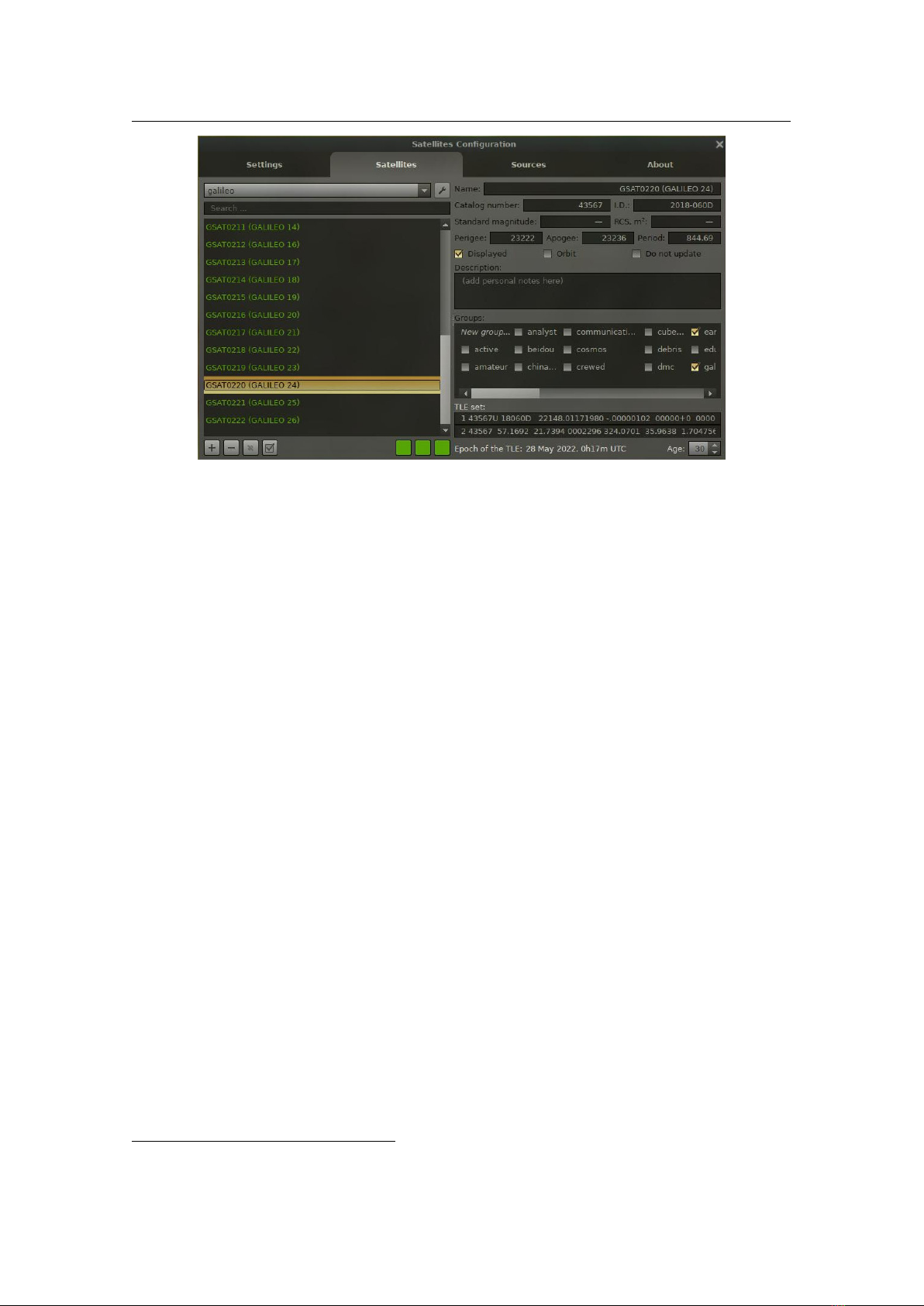
198 Chapter 14. Object Catalog Plugins
Solar longitude
The solar longitude (equinox J2000) gives the position of the Earth on its orbit. It is a more appropriate
information on a meteor shower than the date.
14.6.2 Section
[
MeteorShowers
]
in config.ini file
You can edit
config.ini
file by yourself for changes of the settings for the Meteor Showers plugin – just
make it carefully!
ID Type Description
last_update string Date and time of last update
update_frequency_hours
int Frequency of updates, in hours
updates_enable
bool Enable updates of the meteor showers catalog from Internet
url
string URL of the meteor showers catalog
flag_show_ms_button
bool Enable showing button of the meteor showers on bottom bar
flag_show_radiants
bool Enable displaying markers for the radiants of the meteor showers
flag_active_radiants
bool
Flag for displaying markers for the radiants of the active meteor
showers only
enable_at_startup
bool Enable displaying meteor showers at startup plugin
show_radiants_labels
bool
Flag for displaying labels near markers of the radiants of the meteor
showers
font_size
int
Font size for label of markers of the radiants of the meteor showers
colorARG R,G,B Color for marker of active meteor showers with generic data
colorARR
R,G,B Color for marker of active meteor showers with real data
colorIR
R,G,B Color for marker of inactive meteor showers
14.6.3 Format of Meteor Showers catalog
To add a new meteor shower, you just need to:
1. Copy the code of some valid meteor shower;
2. Paste it in the line 6 (right after the “showers”: {) of the MeteorShowers.json document;
3. Replace the information according with your needs.
Note commas and brackets, they are very important!
" Three - le tter code " :
{
" des ign at ion ": " Name " ,
" IAUNo ": " IAU shower number " ,
" activ ity " :
[{
" year ": " ge neric " ,
" zhr ": Maxim um ZHR ( -1 if v aria ble ) ,
" varia ble " : " Minimum - maxi mum ( if va riab le ) ",
" start ": Solar long itu de at start ,
" finish " : Solar lon git ude at finish ,
" peak ": Solar l ongi tud e at peak ,
" distt ype " : Type of d is tri bu tio n f unct ion
(0= Gauss , 1= Lor entz ) ,
" b1 ": Slope of dist rib ut ion functi on
before peak ,
" b2 ": Slope of dist rib ut ion functi on
after peak
}] ,
" speed ": Ge oce ntr ic speed ( km /s) ,
" rad ia ntA lp ha " : Right A sce nsio n ( J2000 ) ( de gree ) ,
" rad ia ntD el ta " : Decli na tio n ( J2000 ) ( deg ree ) ,
" dri ftA lph a ": Radiant drift in Right Ascension ,
" dri ftD elt a ": Radiant drift in Decli nation ,
" colors " :
[{
" color ": " white " ,
" inte nsi ty " : 70
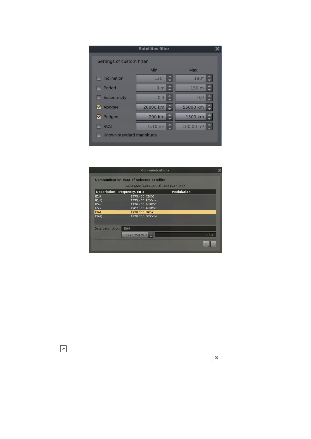
14.6 Meteor Showers Plugin 199
},
{
" color ": " bl ueG ree n ",
" inte nsi ty " : 30
}] ,
" pare ntO bj " : " Pa rent object " ,
" pidx ": popul ati on index
},
For example, below is a record for the Northern Taurids:
" NTA ":
{
" de s i g n a t ion ": " Nort h e rn Tauri d s " ,
" IAUNo ": " 17" ,
" activity " :
[{
" year ": " generi c " ,
" zhr ": 5 ,
" start ": 206 ,
" finis h ": 258 ,
" peak ": 230
}] ,
" speed ": 29 ,
" ra d i a n t A l p h a " : 58 ,
" ra d i a n t D e l t a " : 22 ,
" dr i f tAlpha ": 1.03 ,
" dr i f tDelta ": 0.26 ,
" color s ":
[{
" color ": " yellow " ,
" in tensity ": 80
},
{
" color ": " white " ,
" in tensity ": 20
}] ,
" pa rentObj ": " Come t 2 P /Enc ke " ,
" pidx ": 2.3
},
14.6.4 Notes
•
This plugin uses two models (P. Jenniskens, 1994) and (Peter Jenniskens et al., 1998) to calculate
ZHR, assuming that the activity profile of meteor shower follows a double exponential shape.
•
To predict the local hourly rate, altitude of radiant and limiting magnitude of the sky are taken into
account. Moonlight can also reduce the hourly rate, but is not taken into account.
•
Most of the numerical data for past meteor outbursts (Leonids, etc.) come from (P. Jenniskens, 2006).
There is a wide range of reported values for the maximum ZHR for the 1833 and 1966 Leonids
(P. Brown, 1999). We decided to use a maximum number of 150,000 to demonstrate meteor outbursts
with very high rate.
14.6.5 Further Information
You can get more info about meteor showers here:
•
Wikipedia about Meteor showers: https://en.wikipedia.org/wiki/Meteor_Showers
•
International Meteor Organization: https://www.imo.net/
•
IAU Meteor Data Center: https://www.ta3.sk/IAUC22DB/MDC2007/
Acknowledgements
This plugin was initially created as project of ESA Summer of Code in Space 2013
27
.
27
http://sophia.estec.esa.int/socis2013/?q=about

200 Chapter 14. Object Catalog Plugins
14.7 Navigational Stars Plugin
Figure 14.8: Navigational stars on the screen
This plugin marks navigational stars from a selected set (Figure 14.9):
Anglo-American
— the 57 “selected stars” that are listed in The Nautical Almanac
28
jointly published by
Her Majesty’s Nautical Almanac Office and the US Naval Observatory since 1958; consequently,
these stars are also used in navigational aids such as the 2102-D Star Finder
29
and Identifier.
French
— the 81 stars that are listed in the Ephémérides Nautiques published by the French Bureau des
Longitudes.
Russian — the 160 stars that are listed in the Russian Nautical Almanac.
German
— the 80 stars that are listed in the German Nautical Almanac (The original German title is
Nautisches Jahrbuch) published by the Federal Maritime and Hydrographic Agency of Germany.
If enabled (see section 12.1), just click on the Sextant button on the bottom toolbar to display markers
for the navigational stars. This can help you in training your skills in astronomical navigation before you
cruise the ocean in the traditional way, with your sextant and chronometer.
In the second tab (“Today”, see Figure 14.10) in the plugin’s dialog (right-click the button) you can see
times of sunrise and sunset, twilights, moonrise and moonset.
Civil Twilight
occurs when the zenith angle of the center of the Sun is less than
96
° (
6
° below the horizon)
and the available skylight is still typically sufficient for most civilian outdoor activities. The apparent
horizon is still clearly visible against the glowing sky and only the brightest stars are beginning to
show.
Nautical Twilight
occurs when the zenith angle of the center of the Sun is less than
102
° (
12
° below the
horizon) and the available skylight is no longer sufficient for detailed outdoor activities. However, the
outline of the apparent horizon, as well as most large topographical features, are still distinguishable
and the key stars used for navigational purposes have all typically become visible.
Astronomical Twilight
occurs when the zenith angle of the center of the Sun is less than
108
° (
18
° below
the horizon) and the available skylight is effectively imperceptible compared to moonlight and starlight.
Beyond this angle there is no longer any discernible atmospheric scattering of sunlight, so the time
after astronomical twilight is basically night.
28
The Nautical Almanac website – https://aa.usno.navy.mil/publications/docs/na.php
29
Rude Starfinder 2102-D description and usage instruction –
https://oceannavigation.blogspot.com/200
8/12/rude-starfinder-2102-d.html
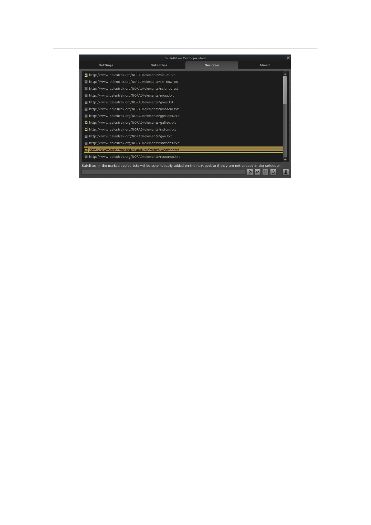
14.7 Navigational Stars Plugin 201
Figure 14.9: Settings of the Navigational stars plugin
Figure 14.10: Today tab in the Navigational stars plugin

202 Chapter 14. Object Catalog Plugins
14.7.1 Section
[
NavigationalStars
]
in config.ini file
You can edit
config.ini
file by yourself for changes of the settings for the Navigational Stars plugin – just
make it carefully!
ID Type Description
navstars_color R,G,B Color of markers of navigational stars
enable_at_startup
bool Set to true to display navigational stars at startup of planetarium
use_utc_time
bool Set to true to use UTC time when navigational stars are displayed
extra_decimals
bool Set to true to show extra decimals in info
upper_limb
bool Set to true to use upper limb for Sun and Moon
tabulated_display
bool Set to true to show information as a tabulated list
limit_info_to_nav_stars
bool
Set to true to show extra information only for marked Navigation
Stars
highlight_when_visible
bool Set to true to highlight only visible stars
current_ns_set
string
Current set of navigational stars. Possible values: AngloAmerican,
French, Russian and German.

14.8 Satellites Plugin 203
14.8 Satellites Plugin
The Satellites plugin displays the positions of artificial satellites in Earth’s orbit based on a catalog of orbital
data. It allows automatic updates from online sources and manages a list of update file URLs.
To calculate satellite positions, the plugin uses an implementation of the SGP4/SDP4 algorithms (J.L.
Canales’ gsat library), using as its input data in NORAD’s two-line element set (TLE
30
) format. Lists with
TLEs for hundreds of satellites are available online and are regularly updated. The plugin downloads the lists
prepared by
https://celestrak.org
to keep itself up-to-date, but the users can specify other sources
online or load updates from local files.
Figure 14.11: Configuration of the Satellites plugin
If the plugin has been enabled (see section 12.1), just click on the Satellite button on the bottom toolbar
to display markers for the satellites, or use right click to call the GUI.
You can search for artificial satellites using the regular search dialog (
F3
). Note that at any given time,
most Satellites will be below the horizon.
Satellites can be either shown as white dots of appropriate brightness similar to moving stars (just like
they appear to the naked eye), or as satellite-shaped markers (icons). Especially this latter view shows
the huge number of satellites in orbit, most of which are invisible to the unaided eye. Satellites which are
v 25.4
reported to transit the penumbra (twilight) zone are rendered with a subdued color.
You can display circles representing the Earth’s shadow (penumbra and umbra, defined just like for Lunar
eclipses, see section 19.11.2), at the altitude of the currently selected satellite, or at a fixed (configurable)
altitude from Earth’s surface.
31
14.8.1 Satellite Properties
Name
Each satellite has a name. It’s displayed as a label of the satellite hint and in the list of satellites.
Names are not unique though, so they are used only for presentation purposes.
Catalog number
In the Satellite Catalog satellites are uniquely identified by their NORAD number, which
is encoded in TLEs.
I.D. (The International Designator)
In the Satellite Catalog satellites are also uniquely identified by their
International Designator also known as COSPAR ID, which is encoded in TLEs.
Standard magnitude
The standard magnitude may be an estimate based on the mean cross-sectional area
derived from its dimensions, or it may be a mean value derived from visual observations (see section
14.8.4).
RCS
The Radar Cross Section is a median value derived from the last several years of values in the Satellite
Situation Report. The units of the RCS are square meters (see section 14.8.4).
Perigee
The perigee is the nearest point respectively of a satellite’s direct orbit around the Earth. The unit
of perigee is kilometers.
30
TLE: https://en.wikipedia.org/wiki/Two-line_element_set
31
The height of the selected satellite is computed above the WGS84 ellipsoid, while the fixed (configurable) altitude
from Earth’s surface is computed over the sphere. You may note these circles will deviate slightly from each other when
displayed altitudes are equal.
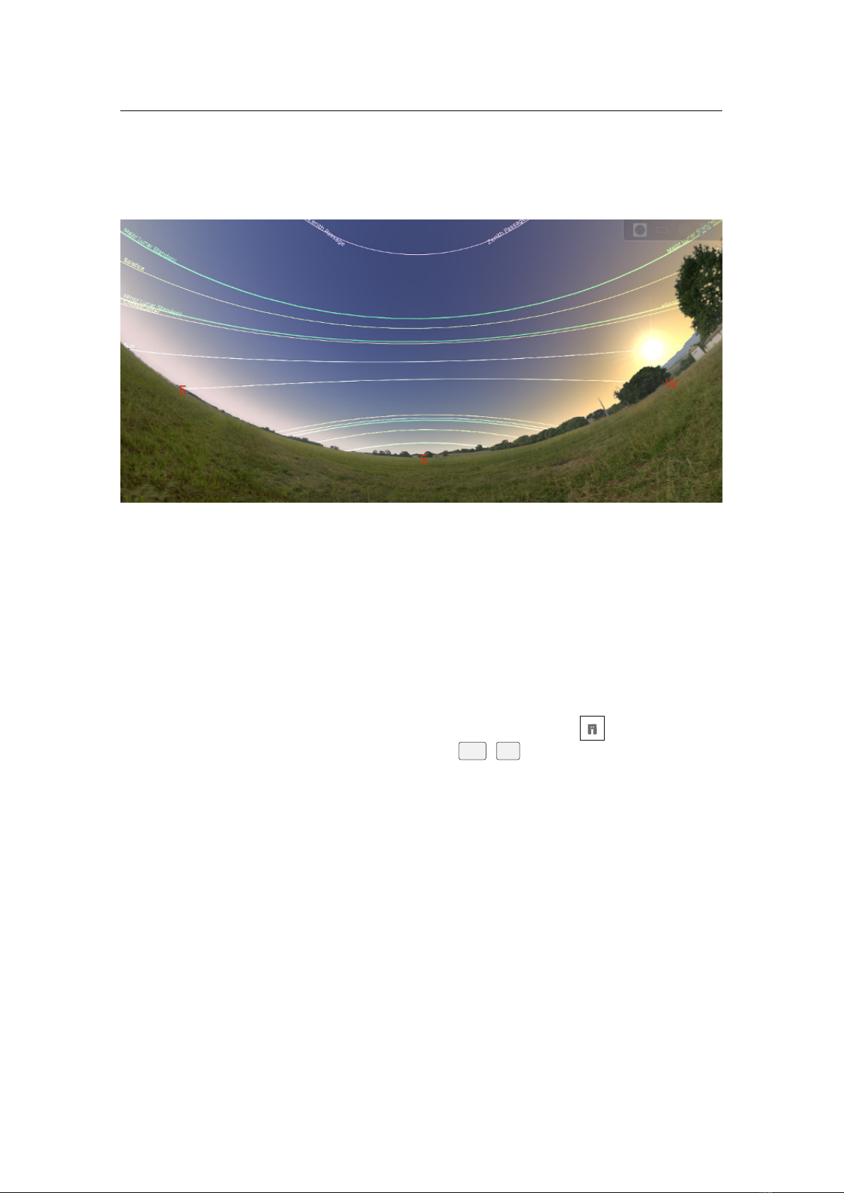
204 Chapter 14. Object Catalog Plugins
Figure 14.12: Configuration of the Satellites plugin: satellite properties
Apogee
The apogee is the farthest point respectively of a satellite’s direct orbit around the Earth. The unit
of apogee is kilometers.
Period
The orbital period is simply how long an orbiting satellite takes to complete one orbit. The unit of
period is minutes.
Displayed
In the Satellite Catalog tab this property controls whether the selected satellite should be
displayed on the sky.
Orbit
In the Satellite Catalog tab this property controls whether the orbit of the selected satellite should be
displayed in the sky.
Do not update
In the Satellite Catalog tab this property marks satellites for which TLE should not be
updated.
Description The user-defined notes for the selected satellite.
Groups
A satellite can belong to one or more groups such as “amateur”, “geostationary” or “navigation”.
They have no other function but to help the user organize the satellite collection. Group names are
arbitrary strings defined in the Satellite Catalog for each satellite and are more similar to the concept
of tags than a hierarchical grouping. A satellite may also not belong to any group at all.
By convention, group names are in lowercase. The GUI translates some of the groups used in the
default catalog.
The group names also can be used as an additional filters for the satellites (see UI elements on the left
side).
TLE set
The raw TLE data of selected satellite. A two-line element set (TLE) is a data format encoding
a list of orbital elements of an Earth-orbiting object for a given point in time, the epoch. Using a
suitable prediction model, the state (position and velocity) at any point in the past or future can be
estimated to some accuracy.
Epoch of the TLE Human-readable epoch of current TLE set.
On the left side of this tab you may see tools for filtering the satellites. The upper part shows a drop-down
list with many predefined filters. Some filters are connected to user defined groups to quickly get a list of
satellites in some group, such as all satellites from group “navigation”. Some filters are connected to orbital
properties of satellites, e.g., selecting the filter “[LEO]” will show all low-orbital satellites.
You can display a list of satellites by specific selection of their properties, when the filter “[custom filter]”
has been selected (Fig. 14.13). The settings of this filter are available through the button
, which is located
at the right of the drop-down list.
You can edit communication data for individual satellites by pressing (Fig. 14.14), where “Descrip-
tion” and “Frequency” are required fields and field “Modulation” is optional. Some individual satellites and
their groups already have the communication data filled in the default catalog.
Abbreviations of some types of modulation:
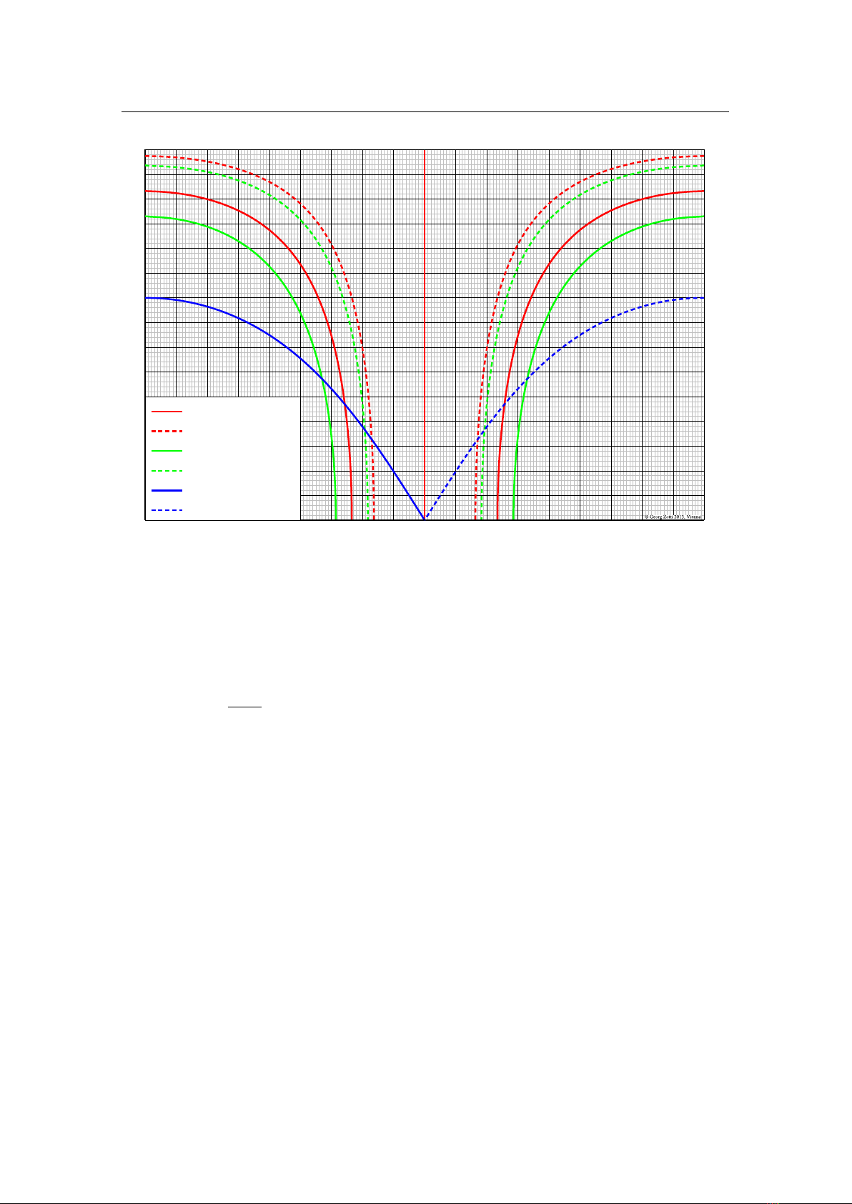
14.8 Satellites Plugin 205
Figure 14.13: Configuration of the Satellites plugin: satellites custom filter
Figure 14.14: Configuration of the Satellites plugin: satellite communication data
APT Automatic Picture Transmission
LRPT Low Resolution Picture Transmission
HRPT High Resolution Picture Transmission
AHRPT Advanced High Resolution Picture Transmission
AX.25 Amateur Radio adaptation of X.25 packet protocol
CW Continuous Wave, Morse Code
AM Amplitude Modulation
FM Frequency Modulation
DUV Data Under Voice
FSK Frequency Shift Keying
GFSK Gaussian Frequency Shift Keying
GMSK Gaussian Minimum Shift Keying
AFSK Audio Frequency Shift Keying
ASK Amplitude-shift Keying
PSK Phase-shift Keying
BPSK Binary Phase-shift Keying
QPSK Quadrature Phase-shift Keying
OQPSK Offset Quadrature Phase-shift Keying
DPSK Differential Phase-shift Keying
BOC Binary Offset Carrier
MBOC Multiplexed Binary Offset Carrier
206 Chapter 14. Object Catalog Plugins
14.8.2 Satellite Catalog
The satellite catalog is stored on disk in JSON
32
format, in a file named
satellites.json
. A default copy
is embedded in the plug-in at compile time. A working copy is kept in the user data directory.
To add a new satellite, open a new line after line 5 and paste the following. Note the structure of commas
and brackets, they are important:
" NORAD num ber ":
{
" name ": " name of the sat e l l ite "
" de s c r i p t ion ": " description goes here ",
" comms ": [
{
" de s c r i p t ion ": " down l i nk 1 " ,
" fr equency ": 437.49 ,
" mo d u lation ": " AFSK 1200 bps "
},
{
" de s c r i p t ion ": " down l i nk 2 " ,
" fr equency ": 145 .825
}
],
" group s ": [ " gro up1 ", " group2 "] ,
" stdMa g ": 2.0 ,
" tle1 ": "1 123 45 U 9 0005 D 09 0 8 0.85236265 .000 0 0 0 14 00000 -0 20602 -4 0 5632 " ,
" tle2 ": "2 123 45 98. 2 700 5 3.2702 0 011918 71.17 76 289.070 5 14 . 3 1 8 1 8920 653 " ,
" visibl e " : true
},
Explanation of the fields:
NORAD number
required parameter, surrounded by double quotes (
"
), followed by a colon (
:
). It is used
internally to identify the satellite. You should replace the text
"NORAD number"
with the first number
on both lines of the TLE set (in this case, "12345"). It must match the number of the satellite in the
source you are adding from if you want the TLE to be automatically updated.
The remaining parameters should be listed between two curly brackets, and the closing curly bracket must be
followed by a comma to separate it from the next satellite in the list:
name
required parameter. It will be displayed on the screen and used when searching for the satellite with
the Find window. Use the description field for a more readable name if you like.
description
optional parameter, double quoted. Appears when you click on the satellite. The description
field can accept HTML tags such as <br/> (new line), <b>bold</b>, etc.
comms optional parameter, square bracketed list of curly bracketed communications information.
groups
optional parameter, comma separated list of double quoted group names contained in square brackets.
Used for grouping satellites in the drop down box on the config (see above)
tle1 required, line 1 of the TLE, must be contained in double quotes and begin with "1 "
tle2 required, line 2 of the TLE, must be contained in double quotes and begin with "2 "
visible
required parameter, set to true if you want to see it, this can be toggled from the configuration
window once the satellite is loaded.
stdMag optional parameter, containing standard magnitude of satellite.
rcs
optional parameter, containing the satellite’s Radar Cross Section. The units of the RCS are square
meters.
You can edit the tags for a satellite, modify the description and comms data, and even add new satellites.
14.8.3 Configuration
The plug-in’s configuration data is stored in Stellarium’s main configuration file.
14.8.4 The approximated visual magnitude
To calculate an approximated visual magnitude of satellites we use the radar cross section (RCS) data and
standard magnitudes from Mike McCants’ database (with permissions)
33
; the radar cross section (RCS) data
from CelesTrack database
34
; the standard magnitudes from database of the MMT-9 observatory (belongs to
32
https://www.json.org/
33
Mike McCants’ Satellite Tracking Web Pages — https://mmccants.org
34
Satellite Catalog (SATCAT) — https://celestrak.org/satcat/search.php
14.8 Satellites Plugin 207
Figure 14.15: Configuration of the Satellites plugin: sources for TLE data
Kazan Federal University) (Beskin et al., 2017; Karpov et al., 2016).
We use a spherical shape of satellite to calculate an approximated visual magnitude from RCS values.
For modelling Starlink visual magnitudes we use Anthony Mallama’s formula
35
(Mallama, 2020) and Mike
McCants’ formula
36
for other satellites.
14.8.5 Sources for TLE data
TLE sets have to be accessed online. Occasionally the source path changes, and configurations set up with
previous versions may no longer be available. Use the bottom right button in the Sources tab (Figure 14.15)
to restore the installation defaults.
Celestrak
37
used as default update source, it also has TLE lists beyond those included by default in Satellite
plug-in
TLE.info
38
Space Track
39
the definitive source, requires sign-up, operated by United States Department of Defense
35
http://www.satobs.org/seesat/Aug-2020/0079.html
36
https://mmccants.org/tles/mccdesc.html
37
https://celestrak.org/NORAD/elements/
38
https://www.tle.info/joomla/index.php
39
https://www.space-track.org/

208 Chapter 14. Object Catalog Plugins
14.9 ArchaeoLines Plugin
GEORG ZOTTI
Figure 14.16: Declination Lines provided by the ArchaeoLines plugin
14.9.1 Introduction
In the archaeoastronomical literature, several astronomically derived orientation schemes are prevalent.
Often prehistorical and historical buildings are described as having been built with a main axis pointing to a
sunrise on summer or winter solstice. There can hardly be a better tool than Scenery3D (see chapter 15) to
investigate a 3D model of such a building, and this plugin has been introduced in version 0.13.3 as a further
tool in the archaeoastronomer’s toolbox (Zotti, 2016b).
When activated (see section 12.1), you can find a a tool bar button (in the shape of a trilithon with
the sun shining through it). Press this, or
Ctrl
+
U
, to display the currently selected set of characteristical
diurnal arcs.
14.9.2 Characteristic Declinations
The ArchaeoLines plugin displays any combination of declination arcs
δ
most relevant to archaeo- or
ethnoastronomical studies. Of course, principles used in this context are derived from natural observations,
and many of these declinations are still important in everyday astronomy.
•
Declinations of equinoxes (i.e., the equator,
δ = 0) and the solstices (δ = ±ε)
•
Declinations of the crossquarter days (days between solstices and equinoxes,
δ(λ = ±45
○
))
•
Declinations of the Major Lunar Standstills (
δ = ±(ε + i))
•
Declinations of the Minor Lunar Standstills (
δ = ±(ε − i))
•
Declination of the Zenith passage (
δ = ϕ)
•
Declination of the Nadir passage (
δ = −ϕ)
•
Declination
δ of the currently selected object
•
Current declination
δ
À
of the sun
•
Current declination
δ
Á
of the moon
•
Current declination
δ
P
of a naked-eye planet
The principal relation between declinations
δ
, geographic latitude
ϕ
, and the rising azimuth
A
is
computed from
cosA = −
sin
δ
cosϕ
. (14.1)
This formula does not take into account local horizon elevation nor atmospheric refraction nor lunar
parallax correction. The effect applied to characteristic declinations is shown graphically for the present time
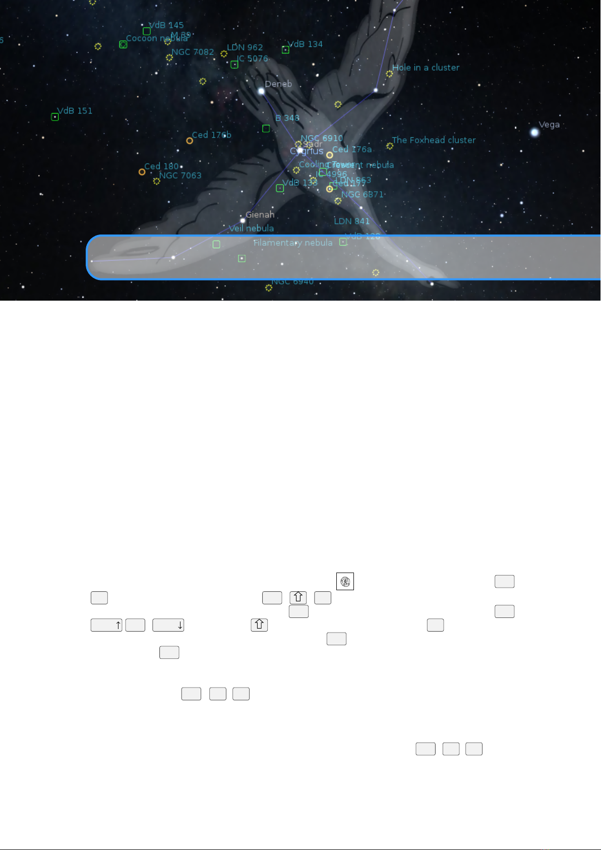
14.9 ArchaeoLines Plugin 209
0 10 20 30 40 50 60 70 80 90 100 110 120 130 140 150 160 170 180
0
5
10
15
20
25
30
35
40
45
50
55
60
65
70
75
0
5
10
15
20
25
30
35
40
45
50
55
60
65
70
75
Solstices, Equinoxes
Solar Crossquarters
Major Standstills
Minor Standstills
Zenith Passage
Nadir Passage
Rising Azimuths, Year 2000
Figure 14.17: Rising azimuths of a few important events for sun and moon, and zenith and nadir
passages depending on geographic latitudes (vertical axis).
(J2000.0) in figure 14.17. For example, in a latitude of 30°, an object which goes through the zenith rises
at azimuth 55°. Lunar major standstill risings occur at azimuths 56.7° and 123.5°, lunar minor standstill
risings at azimuths 69° and 111°. The summer solstice sun rises at 62.6°, the winter solstice sun at 117.3°.
An object which goes through the nadir rises at 125°.
The blue lines seem to vanish at
ϕ = 45
°: while there are still objects going through the zenith in higher
latitudes, they are circumpolar and do not cross the horizon.
For the lunar events, there are two lines each drawn by the plugin, for maximum and minimum distance
of the moon. The lunar extreme declinations are computed taking horizon parallax effects into account.
For technical reasons however, the derived declinations are then used to draw small circles of constant
declinations on the sphere, without taking the change of lunar horizontal parallax into account. Note that
therefore the observed declination of the moon at the major standstill can exceed the indicated limits if it is
high in the sky. The main purpose of this plugin is however to show an indication of the intersection of the
standstill lines with the horizon.
It may be very instructive to let the time run quite fast and observe the declination line of “current moon”
swinging between its north and south limits each month. These limits grow and shrink between the Major
and Minor Standstills in the course of 18.6 years.
The sun likewise swings between the solstices. Over centuries, the solstice declinations very slightly
move as well due to the slightly changing obliquity of the ecliptic.
14.9.3 Geographical Targets
Some religions, e.g., Islam or Bahai, adhere to a practice of observing a prayer direction towards a particular
location. Azimuth lines for two locations can be shown, these lines indicate the great circle direction towards
the locations which can be edited in the configuration window. Default locations are Makkah (the black
Kaaba monument defining prayer direction, or qiblah) and Jerusalem. The azimuth
q
towards a location
T = (λ
T
,
ϕ
T
)
can be computed for an observer at
O = (λ
O
,
ϕ
O
)
based on spherical trigonometry on a spherical
Earth (Abdali, 1997) as
q = arctan
sin(
λ
T
−
λ
O
)
cosϕ
O
tan
ϕ
T
− sin
ϕ
O
cos(
λ
T
−
λ
O
)
(14.2)

210 Chapter 14. Object Catalog Plugins
You can set geographical coordinates and a name label directly, or select locations from Stellarium’s location
list by pressing the
Pick...
button. You can search for locations in the list. When you click on a location,
its data are taken as target, and also distances (angular degrees on a spherical earth, and kilometers on the
v 26.3
flattened earth) are displayed.
14.9.4 Custom Lines
In addition, lines can be shown which indicate arbitrary azimuths (great circles through the zenith), altitudes,
and declinations. Note that these azimuths are always counted from north, regardless of the azimuth setting
described in section 4.3.5. These lines can be marked with a custom label.
When some celestial object is selected, you can take over its current respective data and name by pressing
the button, however the lines are not linked to the selected objects, and changing angle values or time
will make labels invalid.
14.9.5 Configuration Options
The configuration dialog allows the selection of the lines which are of interest to you. In addition, you can
select the color of the lines by clicking on the color swatches.
Section
[
ArchaeoLines
]
in config.ini file
ID Type Default
enable_at_startup bool false
line_thickness
int 1
color_equinox float R,G,B 1.00,1.00,0.50
color_solstices float R,G,B 1.00,1.00,0.25
color_crossquarters float R,G,B 1.00,0.75,0.25
color_major_standstill float R,G,B 0.25,1.00,0.25
color_minor_standstill float R,G,B 0.20,0.75,0.20
color_zenith_passage float R,G,B 1.00,0.75,0.75
color_nadir_passage float R,G,B 1.00,0.75,0.75
color_selected_object float R,G,B 1.00,1.00,1.00
color_current_sun float R,G,B 1.00,1.00,0.75
color_current_moon float R,G,B 0.50,1.00,0.50
color_current_planet float R,G,B 0.25,0.80,1.00
color_geographic_location_1 float R,G,B 0.25,1.00,0.25
color_geographic_location_2 float R,G,B 0.25,0.25,1.00
color_custom_azimuth_1 float R,G,B 0.25,1.00,0.25
color_custom_azimuth_2 float R,G,B 0.25,0.50,0.75
color_custom_altitude_1 float R,G,B 0.25,1.00,0.25
color_custom_altitude_2 float R,G,B 0.25,0.50,0.75
color_custom_declination_1 float R,G,B 0.45,1.00,0.15
color_custom_declination_2 float R,G,B 0.45,0.50,0.65
show_equinox bool true
show_solstices
bool true
show_crossquarters
bool true
show_major_standstills
bool true
show_minor_standstills
bool true
show_zenith_passage
bool true
show_nadir_passage
bool true
show_selected_object
bool true
show_current_sun
bool true
show_current_moon
bool true
show_current_planet string none

14.9 ArchaeoLines Plugin 211
show_geographic_location_1 bool false
show_geographic_location_2
bool false
geographic_location_1_longitude
double 39.826175
geographic_location_1_latitude
double 21.4276
geographic_location_1_name
string Makkah (Qibla)
geographic_location_2_longitude
double 35.235774
geographic_location_2_latitude
double 31.778087
geographic_location_2_name
string Jerusalem
show_custom_azimuth_1 bool false
show_custom_azimuth_2
bool false
custom_azimuth_1_angle
double 0.0
custom_azimuth_2_angle
double 0.0
custom_azimuth_1_label
string custAzi1
custom_azimuth_2_label
string custAzi2
show_custom_altitude_1
bool false
show_custom_altitude_2
bool false
custom_altitude_1_angle
double 0.0
custom_altitude_2_angle
double 0.0
custom_altitude_1_label
string custAlt1
custom_altitude_2_label
string custAlt2
show_custom_declination_1 bool false
show_custom_declination_2
bool false
custom_declination_1_angle
double 0.0
custom_declination_1_label
string custDec1
custom_declination_2_angle
double 0.0
custom_declination_2_label
string custDec2
14.9.6 Acknowledgements
If you are using this plugin in scientific publications, please cite Zotti (2016b).


15. Scenery3d – 3D Landscapes
GEORG ZOTTI AND FLORIAN SCHAUKOWITSCH
15.1 Introduction
Have you ever wished to be able to walk through Stonehenge or other ancient building structures described
as being constructed with astronomical orientation in mind, and experience such orientation in a 3D virtual
environment that also provides a good sky simulation?
The Stellarium Scenery3d plugin allows you to see architectural 3D models embedded in a landscape
combined with the excellent representation of the sky provided by Stellarium. You can walk around, check
for (or demonstrate) possible astronomical alignments of ancient architecture, see sundials and other shadow
casters in action, etc.
15.2 Usage
You activate the plugin with the circular enclosure button at screen bottom or by pressing
Ctrl
+
W
.
A right-click on that button (or
Ctrl
+
+
W
) opens the settings dialog. Once loaded and displaying,
you can walk around pressing
Ctrl
on PC or
Option
on Mac plus cursor keys. Change eye height with
Ctrl
+
Page
/
Ctrl
+
Page
keys on PC or
Option
+
Page
/
Option
+
Page
keys on Mac. Adding
key increases speed by 10, adding
Alt
on PC or
Command
on Mac multiplies by 5 (pressing both keys
multiplies by 50!). If you release
Ctrl
/
Option
before the cursor key, animation will continue. (Press
Ctrl
/
Option
+any cursor key to stop moving.)
Further key bindings exist which can be configured using the Stellarium default key-binding interface.
Some options are also available in the Scenery3d dialog. For example, coordinate display can be enabled
with
Ctrl
+
R
+
T
. If your models are georeferenced in a true geographical coordinate grid, e.g. UTM or
Gauss-Krueger, you will especially like this, and this makes the plugin usable for scientific purposes. Display
shows grid name, Easting, Northing, Altitude of ground, and eye height above ground.
Other features include a virtual “torchlight”, which can be enabled with
Ctrl
+
R
+
L
to give additional
local illumination around the viewer to help to see in the dark. Interesting points of view can be saved and
restored later by the user, including a description of the view. Scene authors can also distribute predefined
viewpoints in their scene.
The plugin also simulates the shadows of the scene’s objects cast by the Sun, Moon and even Venus (only
1 shadow caster used at a time, you will never see shadows cast by Venus in moonlight), so you could use it
for examining sundials, or analyze and simulate light-and-shadow interactions in archaeological structures.
Sometimes, light patches cast through small holes are important, e.g., in churches with meridiana
v 23.2
“sundial/calendar” lines. If these patches appear too dim, you can increase the power of the directional light
using the
Directional light enhancement
switch. (Use value 1.0 to revert to normal.)

214 Chapter 15. Scenery3d – 3D Landscapes
15.3 Hardware Requirements & Performance
In order to work with the non-linear projection models in Stellarium, this plugin uses a trick to create the
foreground renderings: it renders the scene into the six planes of a so-called cubemap, which is then correctly
reprojected onto the sides of a cube, depending on the current projection settings. Your graphics card must
be able to do this, i.e. it must support the OpenGL extension called
EXT_framebuffer_object
. Typical
modern 3D cards (by Nvidia or ATI/AMD) support this extension. In case your graphics hardware does not
support it, the plugin will still work, but you are limited to perspective projection.
You can influence rendering quality, but also speed, using the plugin’s GUI, which provides some options
such as enabling the use of shadows, bumpmapping (provides more realistic surface lighting) or configuring
the sizes of the textures used for the cubemap or shadowmaps. Larger values there improve the quality, but
require faster hardware and more video memory for smooth results.
Because the “cubemap trick” requires quite a large amount of performance (in essence, the scene has to
be rendered 6 times), there are some options available that try to reduce this burden. The first option is to
change the type of the “cubemap”. The most compatible setting is 6 textures, which seems to work best on
older integrated Intel GPUs. The recommended default is the second setting, Cubemap, which uses a more
modern OpenGL feature and generally works a bit faster than 6 textures on more modern graphics cards.
Finally, the Geometry shader option tries to render all 6 cube faces at once. This requires a more recent GPU
+ drivers (at least OpenGL 3.2 must be supported), the setting is disabled otherwise. Depending on your
hardware and the scene’s complexity, this method may give a speedup or may be slower, you must find this
out yourself.
Another option prevents re-rendering of the cubemap if nothing relevant has changed. You can define
the interval (in Stellarium’s simulation time) in which nothing is updated in the GUI. You can still rotate the
camera without causing a re-draw, giving a subjective performance that is close to Stellarium’s performance
without Scenery3d. When moving, the cubemap will be updated. You can enable another option that only
causes 1 or 2 sides of the cubemap to be updated while you move, giving a speedup but causing some parts of
the image to be outdated and discontinuous. The cubemap will be completed again when you stop moving.
Shadow rendering may also cause quite a performance impact. The Simple shadows option can speed
this up a lot, at the cost of shadow quality especially in larger scenes. Another performance/quality factor is
shadow filtering. The sharpest (and fastest) possible shadows are achieved with filtering Off, but depending
on shadowmap resolution and scene size the shadows may look quite “blocky”. Hardware shadow filtering
is usually very fast, but may not improve appearance a lot. Therefore, there are additional filter options
available, the High filter option is relatively expensive. Finally, the PCSS option allows to approximate the
increase of solar and lunar shadow penumbras relative to the distance from their shadow casters, i.e. shadows
are sharp near contact points, and more blurred further away. This again requires quite a bit of performance,
and only works if the shadow filter option is set to Low or High (without Hardware).
The configuration GUI shows tooltips for most of its settings, which can explain what a setting does. All
settings are saved automatically, and restored when you reopen Stellarium.
15.3.1 Performance notes
This plugin clearly runs better with proper 3D graphics cards. On reasonably good hardware (tested on a
notebook PC with Nvidia M960), models with over 10.000.000 triangles are working nicely with shadows
and bumpmaps, although your mileage may vary. On very small hardware like single-board computers
with native OpenGL ES2, models may be limited to 64k vertices (points). If display is too slow, switch to
perspective projection: all other projections require almost sixfold effort! Or try the “lazy” cubemap mode
and lazy updates of tiles, where the scene is only rendered in specific timesteps or when movement happens.
15.4 Model Configuration
The model format supported in Scenery3d is Wavefront .OBJ, which is pretty common for 3D models. You
can use several modeling programs to build your models. Software such as Blender, Maya, 3D Studio Max
etc. can export OBJ.
15.4.1 Exporting OBJ from Sketchup
A simple to use and cost-free modeling program is Sketchup, commonly used to create the 3D buildings
seen in Google Earth. It can be used to create georeferenced models. OBJ is not a native export format for
the standard version of Sketchup. If you are not willing to afford Sketchup Pro, you have to find another
way to export a textured OBJ model.

15.4 Model Configuration 215
Geometry Yes
Lights Yes
Clay No
Photomatched Yes
DefaultUVs No
Instanced No
Table 15.1: Kerkythea Export Settings
One good exporter is available in the Kerkythea renderer project
1
. You need SU2KT 3.17 or better, and
KT2OBJ 1.1.0 or better. Deselect any selection, then export your model to the Kerkythea XML format with
settings shown in 15.1. (Or, with selection enabled, make sure settings are No-Yes-Yes-No-Yes-No-No.)
You do not have to launch Kerkythea unless you want to create nice renderings of your model. Then, use the
KT2OBJ converter to create an OBJ. You can delete the XML after the conversion. Note that some texture
coordinates may not be exported correctly. The setting
Photomatched:Yes
seems now to have corrected
this issue, esp. with distorted/manually shifted textures.
Another free OBJ exporter has been made available by TIG:
OBJexporter.rb
2
. This is the only OBJ
exporter tested so far capable of handling large TIN landscapes (
> 450.000
triangles). As of version 2.6 it
seems to be the best OBJ exporter available for Sketchup.
This exporter swaps Y/Z coordinates, but you can add a key to the config file to correct swapped axes,
see below. Other exporters may also provide coordinates in any order of X, Y, Z – all those can be properly
configured.
Another quirk has to be fixed manually though: in the material description file (MTL), TIG’s exporter
writes both
d
and
Tr
lines with the same value. Actually,
Tr = 1.0− d
according to OBJ/MTL documentation,
so you should edit away one line, or else the later line overwrites the value given earlier. Moreover, given that
Tr=1 should actually specify fully transparent objects, such a line will make your object entirely invisible!
Another (almost) working alternative: ObjExporter.rb by author Honing. Here, export with settings
0xxx00
. This will not create a
TX...
folder but dump all textures in the same directory as the OBJ and
MTL files. Unfortunately, currently some material assignments seem to be bad.
15.4.2 Notes on OBJ file format limitations
The OBJ format supported is only a subset of the full OBJ format: Only (optionally textured) triangle meshes
are supported, i.e., only lines containing statements:
mtllib
,
usemtl
,
v
,
vn
,
vt
,
f
(with three elements
only!), g. Negative vertex numbers (i.e., a specification of relative positions) are not supported.
A further recommendation for correct illumination is that all vertices should have vertex normals.
Sketchup models exported with the Kerkythea or TIG plugins should have correct normals. If your model
does not provide them, default normals can be reconstructed from the triangle edges, resulting in a faceted
look.
If possible, the model should also be triangulated, but the current loader may also work with non-triangle
geometry. The correct use of objects (
o
) and groups (
g
) will improve performance: it is best if you pre-
combine all objects that use the same material into a single one. The loader will try to optimize it anyways if
this is not the case, but can do this only partly (to combine 2 objects with the same material into 1, it requires
them to follow directly after each other in the OBJ). A simple guide to use Blender
3
for this task follows:
1.
File Import Wavefront .obj
- you may need to change the forward/up axes for correct orientation,
try “-Y forward” and “Z up”
2. Select an object which has a shared material
3. Press
+
L
and select ’By Material’
4. Select ’Join’ in the left (main) tool window
5. Repeat for other objects that have shared materials
6.
Export the .obj, making sure to select the same forward/up axes as in the import, also make sure
“Write Normals”, “Write Materials” and “Include UVs” are checked
1
Available at http://www.kerkythea.net/cms/
2
Available from http://forums.sketchucation.com/viewtopic.php?f=323&t=33448
3
https://www.blender.org

216 Chapter 15. Scenery3d – 3D Landscapes
Parameter Default Range Meaning
Ka set to Kd values 0. . . 1 each R/G/B Ambient color
Kd 0.8 0.8 0.8 0. . . 1 each R/G/B Diffuse color
Ke 0.0 0.0 0.0 0. . . 1 each R/G/B Emissive color
Ks 0.0 0.0 0.0 0. . . 1 each R/G/B Specular color
Ns 8.0 0. . . ∞ shinyness
d or Tr 1.0 0. . . 1 opacity
bAlphatest 0 0 or 1 perform alpha test
bBackface 0 0 or 1 render backface
map_Kd (none) filename texture map to be mixed with Ka, Kd
map_Ke (none) filename texture map to be mixed with Ke
map_bump (none) filename normal map for surface roughness
illum 2 integer illumination mode in the standard MTL format.
vis_fadeIn (none) double see 15.4.5
vis_fadeOut (none) double see 15.4.5
Table 15.2: MTL parameters evaluated
For transparent objects (with a
d
or
Tr
value, alpha testing does NOT need this), this recommendation does
NOT hold: for optimal results, each separate transparent object should be exported as a separate “OBJ
object”. This is because they need to be sorted during rendering to achieve correct transparency. If the
objects are combined already, you can separate them using Blender:
1. Import .obj (see above)
2. Select the combined transparent object
3. Enter “Edit” mode with
and make sure everything is selected (press
A
if not)
4. Press
P
and select “By loose parts”, this should separate the object into its unconnected regions
5. Export .obj (see above), also check “Objects as OBJ Objects”
The MTL file specified by
mtllib
contains the material parameters. The minimum that should be specified
is either
map_Kd
or a
Kd
line specifying color values used for the respective faces. But there are other options
in MTL files, and the supported parameters and defaults are listed in Table 15.2.
If no ambient color is specified, the diffuse color values are taken for the ambient color. An optional
emissive term
Ke
can be added, which is modulated to only be visible during nighttime. This also requires
the landscape’s self-illumination layer to be enabled. It allows to model self-illuminating objects such as
street lights, windows etc. It can optionally also be modulated by the emissive texture map_Ke.
If a value for
Ks
is specified, specularity is evaluated using the Phong reflection model
4
with
Ns
as
the exponential shininess constant. Larger shininess means smaller specular highlights (more metal-like
appearance). Specularity is not modulated by the texture maps. Unfortunately, some 3D editors export
unusable default value combinations for
Ks
and
Ns
. Blender may create lines with
Ks
=1/1/1 and
Ns
=0. This
creates a look of “partial overexposed snow fields”. While the values are allowed in the specification, in
most cases the result looks ugly. Make sure to set Ns to 1 or higher, or disable those two lines.
If a value for
d
or
Tr
exists, alpha blending is enabled for this material. This simulates transparency
effects. Transparency can be further controlled using the alpha channel of the map_Kd texture.
A simpler and usually more performant way to achieve simple “cutout” transparency effects is alpha-
testing, by setting
bAlphatest
to 1. This simply discards all pixels of the model where the alpha value of
the
map_Kd
is below the
transparency_threshold
value from
scenery3d.ini
, making “holes” in the
model. This also produces better shadows for such objects. If required, alpha testing can be combined with
“real” blending-based transparency.
Sometimes, exported objects only have a single side (“paper wall”), and are only visible from one side
when looked at in Scenery3d. This is caused by an optimization called back-face culling
5
, which skips
drawing the back sides of objects because they are usually not visible anyway. If possible, avoid such “thin”
geometry, this will also produce better shadows on the object. As a workaround, you can also set
bBackface
to 1 to disable back-face culling for this material.
The optional
map_bump
enables the use of a tangent-space normal maps
6
, which provides a dramatic
4
https://en.wikipedia.org/wiki/Phong_reflection_model
5
https://en.wikipedia.org/wiki/Back-face_culling
6
https://en.wikipedia.org/wiki/Normal_mapping
15.4 Model Configuration 217
improvement in surface detail under illumination.
15.4.3 Configuring OBJ for Scenery3d
The walkaround in your scene can use a ground level (piece of terrain) on which the observer can walk.
The observer eye will always stay “eye height” above ground. Currently, there is no collision detection
with walls implemented, so you can easily walk through walls, or jump on high towers, if their platform
or roof is exported in the ground layer. If your model has no explicit ground layer, walk will be on the
highest surface of the scenery layer. If you use the special name
NULL
as ground layer, walk will be above
zero_ground_height level.
Technically, if your model has cavities or doors, you should export your model twice. Once, just the
ground plane, i.e. where you will walk. Of course, for a temple or other building, this includes its socket
above soil, and any steps, but pillars should not be included. This plane is required to compute eye position
above ground. Note that it is not possible to walk in several floors of a building, or in a multi-plane staircase.
You may have to export several “ground” planes and configure several scenery directories for those rare
cases. For optimal performance, the ground model should consist of as few triangles as you can tolerate.
The second export includes all visible model parts, and will be used for rendering. Of course, this
requires the ground plane again, but also all building elements, walls, roofs, etc.
If you have not done so by yourself, it is recommended to separate ground and buildings into Sketchup
layers (or similar concepts in whichever editor you are using) in order to easily switch the model to the right
state prior to exporting.
Filename recommendations:
<Temple>.skp
Name of a Sketchup Model file. (The
<>
brackets signal “use your own name
here!”) The SKP file is not used by Scenery3d, but you may want to leave it
in the folder for later improvements.
<Temple>.obj Model in OBJ format.
<Temple>_ground.obj Ground layer, if different from Model file.
OBJ export may also create folders
TX_<Temple>
and
TX_<Temple>_ground
. You can delete the folder
TX_<Temple>_ground, <Temple>_ground.obj is just used to compute vertical height.
Put the OBJ, MTL and TX directories into a subdirectory of your user directory (see section 5.1), e.g.
<USERDATA>/Stellarium/scenery3d/<Temple>
, and add a text file into it called
scenery3d.ini
(This
name is mandatory!) with content described as follows.
[model]
name=<Temple>
Unique ID within all models in scenery3d directory. Recommenda-
tion: use directory name.
landscape=<landscapename> Name of an available Stellarium landscape.
This is required if the landscape file includes geographical coordinates and your model does not: First,
the location coordinates of the
landscape.ini
file are used, then location coordinates given here. The
landscape also provides the background image of your scenery. If you want a zero-height (mathematical)
horizon, use the provided landscape called Zero Horizon.
scenery=<Temple>.obj The complete model, including visible ground.
ground=<Temple>_ground.obj Optional: separate ground plane. (NULL for zero altitude.)
description=<Description> A basic scene description (including HTML tags)
The
scenery3d.ini
may contain a simple scene description, but it is recommended to use the localizable
description format: in the scene’s directory (which contains
scenery3d.ini
) create files in the format
description.<lang>.utf8
which can contain arbitrary UTF-8–encoded HTML content.
<lang>
stands
for the ISO 639 language code.
author=<Your Name yourname@yourplace.com>
copyright=<Copyright Info>
obj_order=XYZ
Use this if you have used an exporter which swaps Y/Z coordinates.
Defaults to XYZ, other options: XZY, YZX, YXZ, ZXY, ZYX
camNearZ=0.3
This defines the distance of the camera near plane, default 0.3.
Everything closer than this value to the camera can not be displayed.
Must be larger than zero. It may seem tempting to set this very
small, but this will lead to accuracy issues. Recommendation is
not to go under 0.1
camFarZ=10000 Defines the maximal viewing distance, default 10000.
218 Chapter 15. Scenery3d – 3D Landscapes
shadowDistance=<val>
The maximal distance shadows are displayed. If left out, the value
from
camFarZ
is used here. If this is set to a smaller value, this
may increase the quality of the shadows that are still visible.
shadowSplitWeight=0..1
Decimal value for further shadow tweaking. If you require better
shadows up close, try setting this to higher values. The default is
calculated using a heuristic that incorporates scene size.
[general]
The general section defines some further import/rendering options.
transparency_threshold=0.5
Defines the alpha threshold for alpha-testing, as described in sec-
tion 15.4.2. Default 0.5
scenery_generate_normals=0
Boolean, if true normals are recalculated by the plugin, instead of
imported. Default false
ground_generate_normals=0 Boolean, same as above, for ground model. Default false.
[location]
Optional section to specify geographic longitude
λ
, latitude
ϕ
, and altitude. The section is required if
coord/convergence_angle={from_grid|from_utm}, else location is inherited from landscape.
planet = Earth
latitude = +48d31’30.4" Required if coord/convergence_angle=from_{grid|utm}
longitude = +16d12’25.5" "–"
altitude =from_model|<int>
altitude (for astronomical computations) can be computed from the
model: if
from_model
, it is computed as
(z
min
+ z
max
)2+ orig_H
,
i.e. from the model bounding box centre height.
display_fog = 0
atmospheric_extinction_coefficient = 0.2
atmospheric_temperature = 10.0
atmospheric_pressure = -1
light_pollution = 1
[coord]
Entries in the
[coord]
section are again optional, default to zero when not specified, but are required if
you want to display meaningful eye coordinates in your survey (world) coordinate system, like UTM or
Gauss-Krüger.
grid_name=<string>
Name of grid coordinates, e.g.
"UTM 33 U (WGS 84)"
,
"Gauss-Krüger M34"
or
"Relative to <Center>"
This name is only displayed, there is no evaluation of its
contents.
orig_E=<double> | (Easting) East-West-distance to zone central meridian
orig_N=<double> | (Northing) North distance from Equator
orig_H=<double> | (Height) Altitude above Mean Sea Level of model origin
These entries describe the offset, in metres, of the model coordinates relative to coordinates in a geographic
grid, like Gauss-Krüger or UTM. If you have your model vertices specified in grid coordinates, do not specify
orig_... data, but please definitely add start_... data, below.
Note that using grid coordinates without offset for the vertices is usually a bad idea for real-world
applications like surveyed sites in UTM coordinates. Coordinate values are often very large numbers
(ranging into millions of meters from equator and many thousands from the zone meridian). If you want to
assign millimetre values to model vertices, you will hit numerical problems with the usual single-precision
floating point arithmetic. Therefore we can specify this offset which is only necessary for coordinate display.
Typically, digital elevation models and building structures built on those are survey-grid aligned, so true
geographical north for a place with geographical longitude
λ
and latitude
ϕ
will in general not coincide with
grid north, the difference is known as meridian convergence
7
and, on a spherical globe, amounts to:
γ(λ , ϕ)= arctan(tan(λ − λ
0
)sin
ϕ) (15.1)
7
https://en.wikipedia.org/wiki/Transverse_Mercator_projection
15.4 Model Configuration 219
This amount can be given in convergence_angle (degrees), so that your model will be rotated clockwise
by this amount around the vertical axis to be aligned with True North
8
.
co nverg ence_ angle = from_grid | from _utm |<double >
gr id_ merid ian = < double >|+ < int >d < int > ’< float >"
grid_meridian
is the central meridian
λ
0
of the grid zone, e.g. for Gauss-Krüger, and is only required to
compute convergence angle if
convergence_angle=from_grid
. If your model coordinates is based on
UTM, you can use coord/convergence_angle=from_utm for a more accurate computation.
ze ro_gr ou nd_he ight =< double >
height of terrain outside
<Temple>_ground.OBJ
, or if
ground=NULL
. Allows smooth approach from
outside. This value is relative to the model origin, or typically close to zero, i.e., use a Z value in model
coordinates, not world coordinates! (If you want the terrain height surrounding your model to be
orig_H
,
use 0, not the correct mean height above sea level!) Defaults to minimum of height of ground level (or model,
resp.) bounding box.
start_E=<double>
start_N=<double>
start_H=<double> only meaningful if ground==NULL, else H is derived from ground
start_Eye=<double> default: 1.65m
start_az_alt_fov=<az_deg>,<alt_deg>,<fov_deg>
initial view direction and field of view.
start_...
defines the view position to be set after loading the scenery. Defaults to center of model
boundingbox.
It is advisable to use the grid coordinates of the location of the panoramic photo (landscape) as
start_...
coordinates, or the correct coordinates and some carefully selected
start_az_alt_fov
in case you want to
highlight a certain view corridor (temple axis, . . . ).
In some setups like digital full-dome planetaria it is advisable to disable the use of the
start_az_alt_fov
.
v 23.2
You can do that in the Scenery3D configuration dialog or by the entry
ignore_start_az_alt_fov
in
config.ini.
15.4.4 Concatenating OBJ files
Some automated workflows may involve tiled landscape areas, e.g. to overcome texture limitations or
triangle count limits in simpler tools like Sketchup. In this case you can create separate meshes in the same
coordinate system, but you need to concatenate them. One powerful program to assemble your parts is again
Blender.
In Blender, import the OBJ files
File Import Wavefront .obj
. If your OBJ coordinates have Z as
vertical axis (common for terrestrial models), use “Z up”, “-Y Forward” as import settings for the coordinate
axes. The model will appear south-up.
Blender may not show anything except the default cube because of aggressive camera far plane clipping.
Press
N
and in the
View
set at least the far clipping plane as required to see the full extent of your terrain
model. Then press
View View All
(or
Home
).
The landscape may look white now. Switch on textured view if required (
Alt
+
Z
). If the scene looks
almost black now, reconfigure the light to be sunlight: Select the lamp in the outliner graph, press the lamp
icon and in the
Lamp
select “Sun”. Now the scene should be in full color, and the Y axis should point
towards grid-south.
After importing the first model, you may consider locking it in place to avoid errors. Select the model in
the outliner, select the cube button below, then open
Transform Locks
and lock all. The other model parts may
have to be transformed, and numerical transformation can be added in the
Transform
settings in this menu.
If you have created a VRML (WRL) of some structures in ArcScene, export that without shifting to
center, and import the WRL file in Blender with default orientation “Y up”, “Z forward”. Models from other
sources may still be different.
In the end, all parts should fit neatly together. Blender is a very powerful program, you can enhance
your model as you wish.
8
Note that Sketchup’s georeferencing dictionary provides a NorthAngle entry, which is
360− convergence_angle
.

220 Chapter 15. Scenery3d – 3D Landscapes
When the model configuration is complete, select all relevant parts which you want to have visible in
Stellarium (click on the lines in the outline view containing the object names to light them up gray, then
Rightclick-Select, so that the triangle (mesh) icon has a colored background circle) and press
Ctrl
+
J
to
optionally join them, then export to a single OBJ
File Export Wavefront .obj
. In the export options, apply
“Selection Only”, and “-Y Forward” and “Z Up”
9
.
Verify the new model loads correctly, e.g. in Meshlab
10
!
15.4.5 Beyond 3D: Temporally evolving Models
Stellarium working as “time machine” can display the sky for any calendar date in its range of valid dates.
Also landscapes and human-built structures evolve. Temples are being rebuilt, changed, re-dedicated or
repurposed, new windows are cut, old windows closed. To show landscape and buildings in the right shape
for the time in question, we can make material transparent, so that parts of the model are not displayed. To
allow for archaeological uncertainties in dating construction and destruction, we can gradually fade in and
fade out the model parts in question (Zotti, Schaukowitsch, and Wimmer, 2018).
To enable this magic, you must combine all your models into one (see section 15.4.4), export as one
OBJ/MTL as usual, and manually edit the MTL file. It is wise to give the material for the parts in question a
reasonable name that you can later identify in the MTL file. Then you simply add one or both of the new
keywords
vis_fadeIn
or
vis_fadeOut
to the material description, with 2 arguments which are the Julian
days of begin and end of a phase transition. For sharp transitions, just use the same JD dates.
# Some str ucture has been put up around -3100/ -3000
vis_fadeIn 58 8783.5 625 308.5
# Fade away between 500 AD /700 AD
vis_f ade Out 190 368 2.5 19 76732.5
15.4.6 Working with non-georeferenced OBJ files
There exists modeling software which produces nice models, but without concept of georeference. One
spectacular example is AutoDesk PhotoFly, a cloud application which delivers 3D models from a bunch of
photos uploaded via its program interface. This “technological preview” is in version 2 and free of cost as of
mid-2011.
The problem with these models is that you cannot assign surveyed coordinates to points in the model, so
either you can georeference the models in other applications, or you must find the correct transformation
matrix. Importing the OBJ in Sketchup may take a long time for detailed photo-generated models, and the
texturing may suffer, so you can cut the model down to the minimum necessary e.g. in Meshlab, and import
just a stub required to georeference the model in Sketchup.
Now, how would you find the proper orientation? The easiest chance would be with a structure visible in
the photo layer of Google Ear th. So, start a new model and immediately
add location
from the Google
Earth interface. Then you can import the OBJ with TIG’s importer plugin. If the imported model looks
perfect, you may just place the model into the Sketchup landscape and export a complete landscape just
like above. If not, or if you had to cut/simplify the OBJ to be able to import it, you can rotate/scale the OBJ
(it must be grouped!). If you see a shadow in the photos, you may want to set the date/time of the original
photos in the scene and verify that the shadows created by Sketchup illuminating the model match those in
the model’s photo texture. When you are satisfied with placement/orientation, you create a
scenery3d.ini
like above with the command
Plugins ASTROSIM/Stellarium scenery3d helpers Create scenery3d.ini
.
Then, you select the OBJ group, open the
Windows Ruby Console
and readout data by calling
Plugins
ASTROSIM/Stellarium scenery3d helpers Export transformation of selected group
.
On the Ruby console, you will find a line of numbers (the
4 × 4
transformation matrix) which you
copy/paste (all in one line!) into the [model] section in scenery3d.ini.
ob j2grid_t rafo = <a11 >, < a12 >, < a13 >,< a14 >,< a21 >,< a22 >,<a23 >, <a24 >,
<a31 >,< a32 >,< a33 >,< a34 >,< a41 >,< a42 >,< a43 >,< a44 >
You edit the
scenery3d.ini
to use your full (unmodified) PhotoFly model and, if you don’t have a
panorama, take
Zero Horizon
landscape as (no-)background. It depends on the model if you want to be
9
https://blender.stackexchange.com/questions/3352/merging-multiple-obj-files
10
https://www.meshlab.net/

15.5 Predefined views 221
able to step on it, or to declare
ground=NULL
for a constant-height ground. Run Stellarum once and adjust
the start_N, start_E and zero_ground_height.
15.4.7 Rotating OBJs with recognized survey points
If you have survey points measured in a survey grid plus an image-based model with those points visible,
you can use Meshlab to find the model vertex coordinates in the photo model, and some other program
like CoordTrans in the JavaGraticule3D suite to find either the matrix values to enter in
scenery3d.ini
or even rotate the OBJ points. However, this involves more math than can be described here; if you came
that far, you likely know the required steps. Here it really helps if you know how to operate automatic text
processors like AWK.
15.5 Predefined views
You can also configure and distribute some predefined views with optional date of interest with your model
in a
viewpoints.ini
file. The viewpoints can be loaded and stored with the viewpoint dialog which you
can call with the button. See the provided “Sterngarten” scene for an example. These entries are not
editable by the user through the interface. The user can always save his own views, they will be saved into
the file userviews.ini in the user’s Stellarium user directory, and are editable.
[ St o r e d V i ews ]
size =< int > D efines how many entrie s are in this file .
Pr efix each ent ry with its index !
1/ label =< string > The name of this entry
1/ description =< string > A de s c r i p tion of thi s entry ( can in c l ude HTML )
1/ positi o n =<x , y ,z ,h > The x ,y ,z grid coordinates
( like orig_ * or s tart_ * in s c e nery3d . ini )
+ the curre n t eye height h
1/ view_f o v =< az_deg , alt_deg , fov_deg > The view d irection + FOV
( like start_ a z _ a l t _ f o v in scener y 3 d . ini )
; an exampl e for a sec ond entry ( note the 2 at the begin n i n g of each line !)
2/ label = Signs
2/ description = Two signs that des c ribe the St e r n g a rten
2/ positi o n = 59 3 1 5 5 . 2421 ,5333348.6304 ,325.729 5 8 0 9 0 3 8 , 0 . 8 8 0 5
2/ view_f o v = 8 4 .31539 9 , -8. 187078 ,83.00 0 000
2/ JD = 2 4 51545.5 [ op t ional ]
15.6 Example
Let us add a quick example here. A recent paper (Pollard, 2017) claims that the Uffington White Horse, a
geoglyph carved into a hillsite in England during the Bronze Age, may depict the mythical “Sun Horse”, a
common conception of that period.
Unfortunately, as of 2017, the official UK Lidar repository does not include the Uffington area, so a
detailed GIS-based model is not available. We could use EUdem25 data with aerial imagery, or for a quick
look, we just use Sketchup. Yet another unfortunate development: Trimble declared that after the 5-year
transition period from Google to Trimble is over in May 2017, terrain modelling will be limited to Sketchup
Pro. But note that a fresh installation comes with a 30-day Pro trial time, this should be enough for this
example.
First, locate the site in Google Earth at
λ = −1.56718, ϕ = 51.582843
. (Or just search for “Uffington”.)
Try to identify which parts of the landscape may be visible from your site, so you can estimate which parts
of terrain should be included in the model. Open Sketchup, select the meter-based “Landscape Architecture”
template, add
View Toolbars. . .
: Locations. Click on the “Add Location” button of that toolbar. Enter
“Uffington” into the location search dialog. This brings you close to our site of interest. Clip a part of terrain
to import it to Sketchup. Optionally, add more terrain.
If installed, TIG’s OBJ exporter is available from the
File
menu, or you can use Sketchup Pro’s
built-in OBJ export. Export
UffingtonHorse.obj
to a subdirectory
scenery3d/Uffington
in your
Stellarium user data directory. The geolocation is stored in an “AttributeDictionary”. To read this, press
Window Ruby Console
to open the Ruby Console. Then write a few lines of Ruby to get access to the
Georeference dictionary and other data:
model = Sketchup . ac tive _model
attrdic ts = model . at tribute _dictio na ries

222 Chapter 15. Scenery3d – 3D Landscapes
attrdic ts . each {| d|
puts " Attr ibuteDi ction ar y : % s" % d. name
d. each _pair { |k , v | puts " %s =% s" % [k, v] }
}
model . shadow_ inf o . each {|k, v| puts " #{ k } #{ v} "}
utm = model . point_t o_ut m Geom :: Point3d . new (0 ,0 ,0)
puts ( " grid_name = UTM %i % s (% s)" %
[ utm . zone_number , utm . zone_letter , model . get_datum ])
Note the
ModelTranslation
values. Those are inches (of all units!) in the UTM reference frame and
define the model coordinate origin in world coordinates. (Actually, it uses the negative values.) Multiplication
by 2.54 gives cm, and by 0.0254, meters in the UTM coordinate system. We will use the negatives of these
values as
orig_E
,
orig_N
,
orig_H
. Additionally, we have found information about meridian convergence
correction (Sketchup’s
NorthAngle
), UTM zone number etc. All this goes into our configuration file.
Create this file scenery3d.ini with the content seen in fig. 15.1
15.7 Limitations
Models with up to 14 million triangles have been used successfully on a mid-range notebook PC from 2016.
However, take some restrictions into account:
•
The model is rendered in Cartesian coordinates. Earth’s surface is curved. If your model extends by
tens of kilometres, the visible horizon formed by faraway mountains may appear too high. You can
display a landscape polygon defined in the currently displayed Landscape on top of your 3D scene by
activating
Draw horizon polyline in foreground
in the plugin’s settings dialog.
•
The OBJ format is static. Simulation of interaction with 3D objects is not possible with this plugin.
Authors and Acknowledgements
Scenery3d was conceived by Georg Zotti for the ASTROSIM
11
project. A first prototype was implemented in
2010/2011 by Simon Parzer and Peter Neubauer as student work supervised by Michael Wimmer (TU Wien).
Models for accuracy tests (Sterngarten, Testscene), and later improvements in integration, user interaction,
.ini option handling, OBJ/MTL loader bugfixes and georeference testing by Georg Zotti.
Andrei Borza in 2011/12 further improved rendering quality (shadow mapping, normal mapping) and
speed (Zotti, 2015; Zotti and Neubauer, 2012a; Zotti and Neubauer, 2012b).
In 2014–17, Florian Schaukowitsch adapted the code to work with Qt 5 and the Stellarium 0.13 codebase,
replaced the renderer with a more efficient, fully shader-based system, implemented various performance,
quality and usability enhancements, and did some code cleanup. Both Andrei and Florian were again
supervised by Michael Wimmer (Zotti, 2016a; Zotti, 2016b; Zotti, Schaukowitsch, and Wimmer, 2018).
This work has been originally created during the ASTROSIM project supported 2008-2012 by the
Austrian Science Fund (FWF) under grant number P 21208-G19. Further development has partially been
supported by the Ludwig Boltzmann Institute for Archaeological Prospection and Virtual Archaeology in
Vienna, Austria
12
.
If you are using this plugin in scientific work, please cite: (Zotti, 2016a; Zotti, 2016b; Zotti, 2019; Zotti,
Frischer, et al., 2019; Zotti, S. Hoffmann, et al., 2021; Zotti, Schaukowitsch, and Wimmer, 2018).
11
https://astrosim.univie.ac.at
12
https://archpro.lbg.ac.at
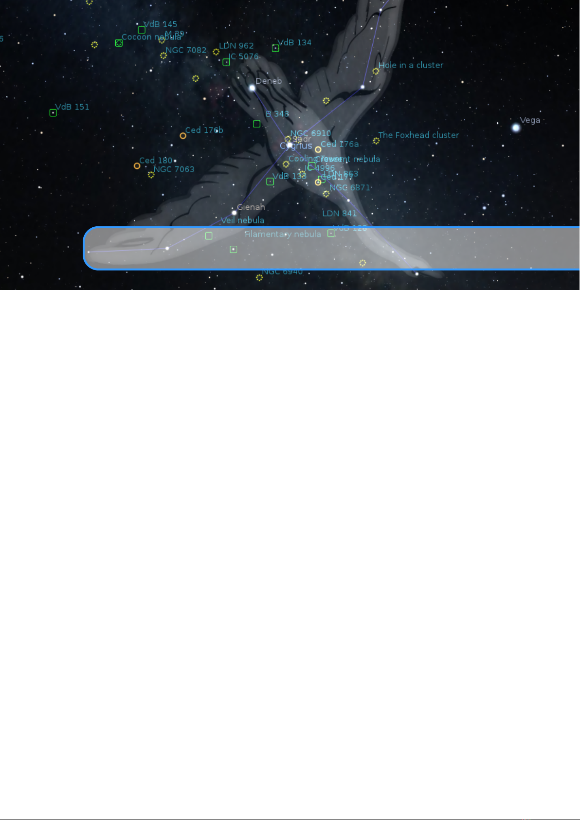
15.7 Limitations 223
[ model ]
name = Uffi ngton Horse
; Either a fitting landscape or just ’ Zero Hori zon ’:
landsca pe = Zero Horizon
scener y = Uffin gtonH orse . obj
; activate the next line if you have a separa te ground layer
; ground = Uf fington Horse_g ro und . obj
; If model Y - axis points up , activate the next line
; obj_order = XZY
author = Georg Zotti
copyrig ht =( c) 2017 Georg Zotti
descr ipt ion = Uffington Horse may represent the Sun Horse . \
See Joshua Pollar d in An tiquity 91 356(2 017 ): 406 -20.
[ location ]
name = Uffi ngton Horse
countr y = UK
planetName = Earth
; Set the fol low ing to a fitt ing land sca pe
lands cape Key = Zero Hor izon
longitu de = -1.5 67182540893 55
lati tude = 51.58 28432 74982 3
alti tude =137
[ coord ]
grid_na me = UTM 30 U ( WGS 84)
grid Type = UTM
orig_E =59927 3.021 19578
orig_N = 57156 15.15 07910 6
orig_H = 136.2 95297 62673 6
co nverg ence_ angle = 1.122 84363 77198 8
; Height used outside the terrain , to not " fall off " the rim .
ze ro_gr ou nd_he ight =137
; You may want to reset these co ord inat es .
; Observer is set to those on loading the scenery .
start_ E = 59927 3.021 19578
start_ N = 57156 15.15 07 9106
st art_a z_alt _fov =50 ,10 ,83
Figure 15.1: scenery3d.ini for the Uffington example.
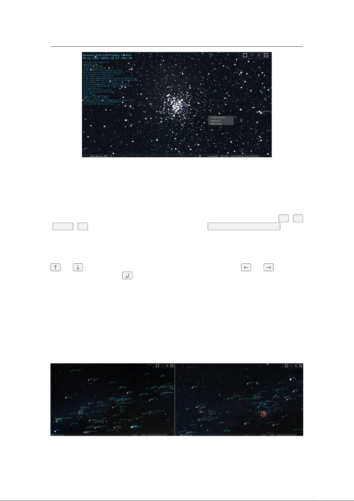
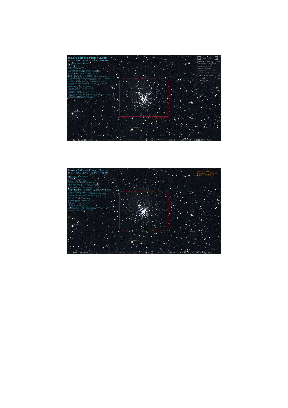
16. Stellarium at the Telescope
Stellarium is great for indoor use on the desktop, but it is also very useful outdoors under the real sky, and
several plugins enhance its usability particularly for observers.
Right at the telescope, Oculars (section 16.1) provides field of view hints for telescopes, oculars and
sensors, and TelescopeControl (section 16.2), which allows you to send GOTO commands to most motorized
telescope mounts. Other GOTO telescopes are supported by external programs which you must install
separately: RTS2 (16.2.6), INDI (16.2.7) or ASCOM (16.2.8). This can also help DIY hardware tinkerers who
like to build their own control systems (section 16.2.10).
In addition, the Observability plugin (16.3) can be used for planning the best times to observe your
favorite objects, and the Mosaic Camera plugin (16.4) can be used to show the orientations of more
complicated camera mosaics.
16.1 Oculars Plugin
TIMOTHY REAVES, WITH ADDITIONS BY ALEXANDER WOLF
This plugin serves several purposes:
•
to see what the sky looks like through a particular combination of eyepiece, lens (Barlow or Shapley
types) and telescope. This plugin helps to get an idea of what you should see when looking through
a physical telescope, and understand why one eyepiece may be better suited to observe a particular
target than another. This can also be very useful for deciding what telescope is best suited to a style of
viewing. And with the support for binoculars, you also have the ability to understand just about any
type of optics-enhanced visual observing.
•
to show what a particular combination of camera and telescope (or photographic lens) would be able
to photograph of the sky.
•
lastly, with the help of the Telrad sight, understand where object in the sky are in relation to each
other. This can be helpful for star-hopping with a non-GOTO telescope.
None of these activities can take the place of hands-on experience, but they are a good way to supplement
your visual astronomy interests.
16.1.1 Using the Ocular plugin
The plugin is controlled through a popup menu or through an on-screen control panel (see top right corner
on screens in fig. 16.17). By default, the hot key to display the popup is
Alt
+
O
(
Option
+
O
for Mac
users). This can be changed in the
Editing Keyboard Shortcuts
window (see section 4.8). The menu will
popup where your cursor is located.
The options available in the popup menu depend on what you are currently doing. In the default menu,
you can choose to configure the plugin, activate a CCD, or activate the Telrad finder (see fig. 16.1). The
menu is navigated by either the arrow keys on your keyboard or by your mouse. The
and arrow
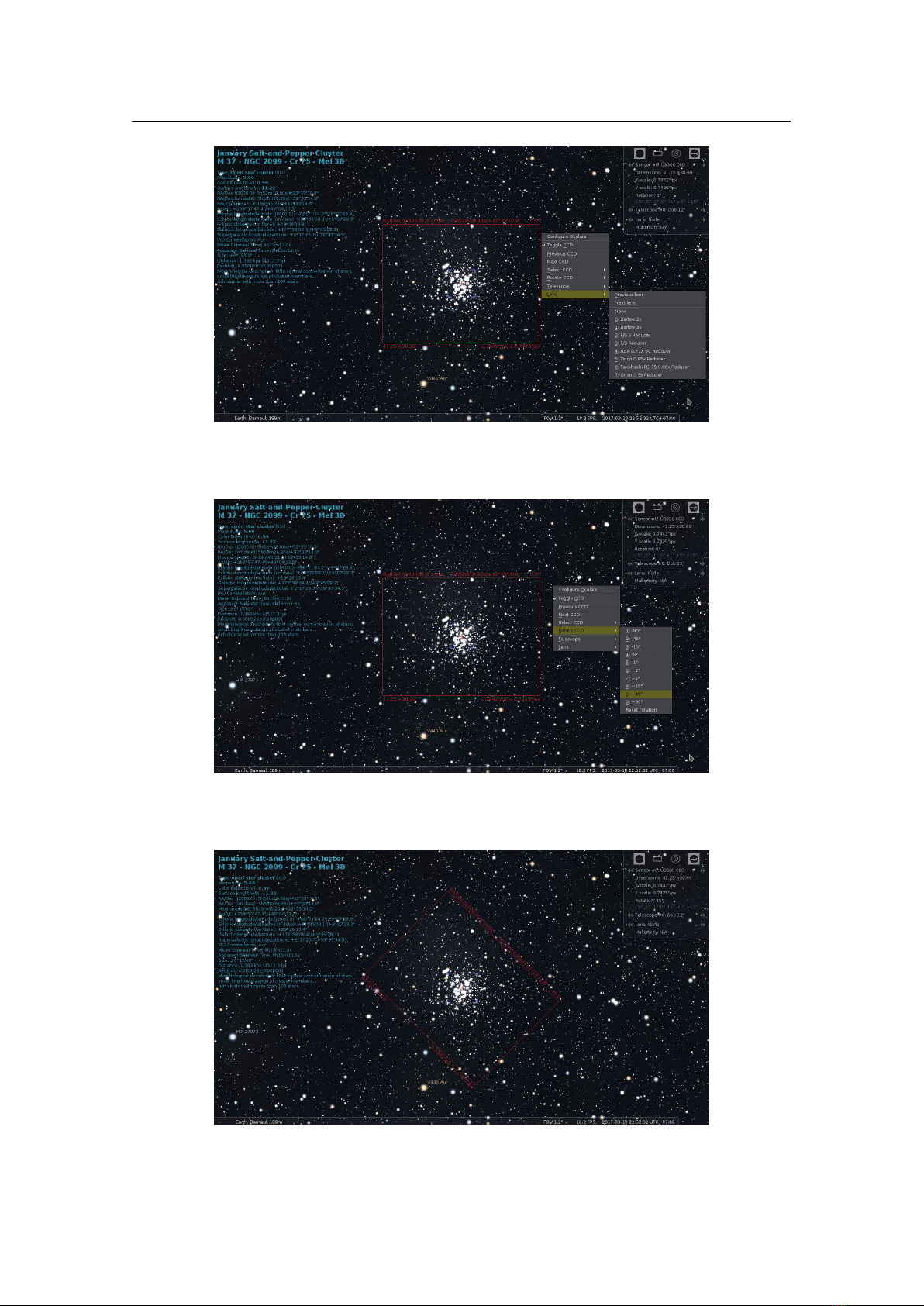
226 Chapter 16. Stellarium at the Telescope
Figure 16.1: The on-screen menu (top right) and popup menu (lower right) of the Oculars plugin.
keys move the selection up or down the menu, and the and arrow keys display or hide sub-menus.
activates an option.
Telrad Finder
The Telrad view can be used without defining any of the items below. As a reflex sight is non-magnifying,
this feature can only be enabled when no eyepiece is selected. You still may want to zoom in a bit to better
see which stars are in the circles (fig. 16.2). The three circles that appear in the center of the screen are
0.5
°,
2.0
°, and
4.0
° in diameter. They stay centered in the screen, so move the “telescope” (click-drag the
background) to center the circles on the object of interest.
While the Telrad finder is active, you can not activate a CCD with the popup menu, but only with the
on-screen menu.
CCD Sensors
This is a great way to get an idea of what a particular camera will be able to capture when attached to a
particular telescope or lens. For using camera lenses, describe them as telescope with the appropriate values
for the lens. When active, this feature will display a red bounding box of the area that will be captured, as
well as zoom in to give a better view of the surroundings. You can manually zoom in or out from there.
The default CCD view will appear similar to fig. 16.3 or, when you are working without the on-screen
control panel, the information area in the upper right hand corner also shows angular size captured by the
CCD (see fig. 16.4).
When a CCD view is displayed, the popup menu changes as seen in fig. 16.5. You can select what
telescope to use, as well as progress to the previous or next CCD, or go to a specific CCD. You can also
rotate the CCD to better frame your subject, or to see if the CCD can be rotated in such a way as to catch
your area of interest (see fig. 16.6). Once rotated, the CCD frame on screen displays the new orientation (see
fig. 16.7).
Figure 16.2: The left image is the default 60°, and the right one is 40°.
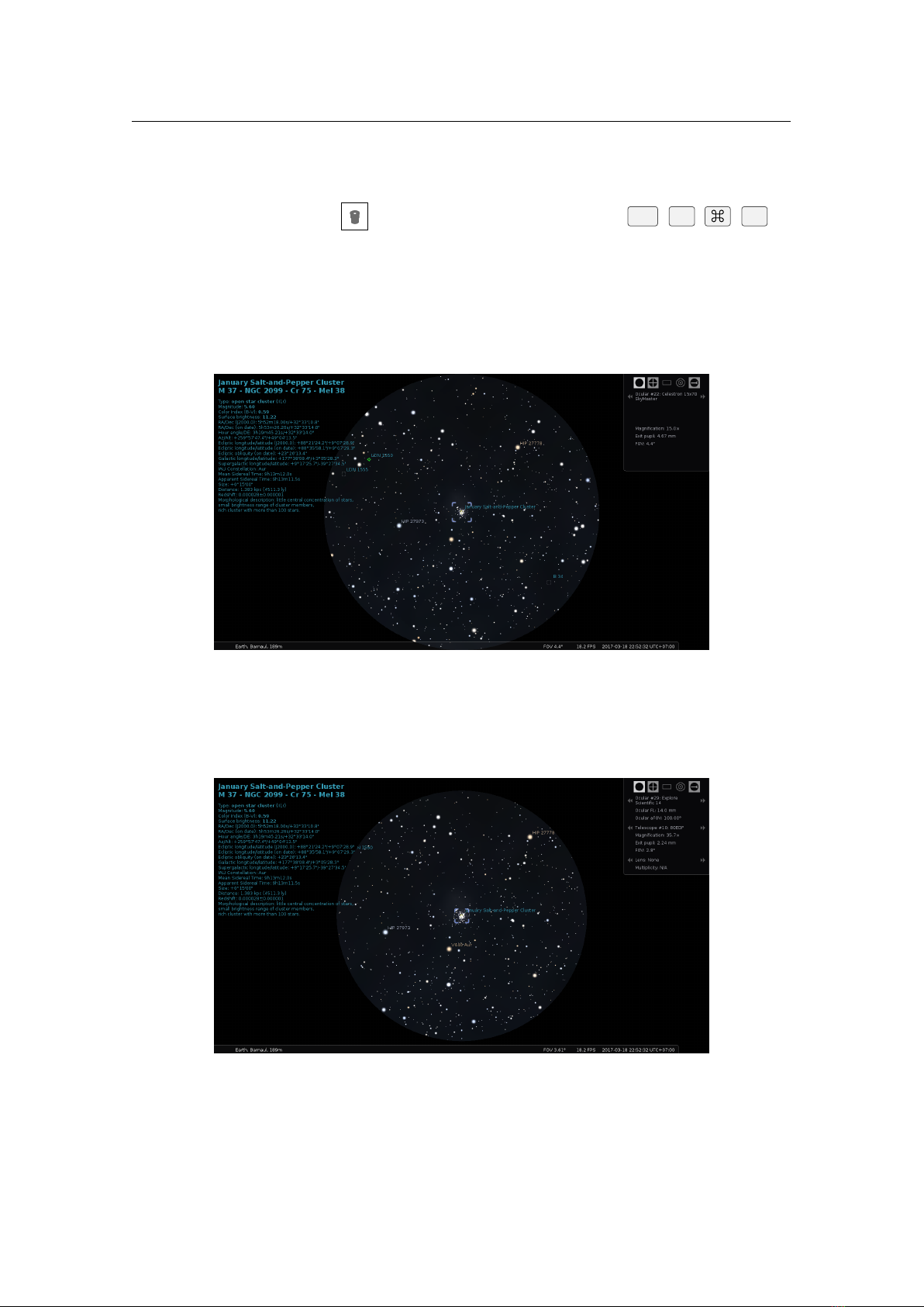
16.1 Oculars Plugin 227
Figure 16.3: View of M37 through a CCD sensor of the Oculars plugin.
Figure 16.4: View of M37 through a CCD sensor of the Oculars plugin (without on-screen control
panel).
Oculars
•
Define some eyepieces and telescope (see section 16.1.2).
•
Select an object to view (i.e. a star, planet, etc.)
•
Click the toolbar button for toggling the Ocular view, or press
Ctrl
+
O
(
+
O
for Mac
users).
•
Swap between eye pieces and telescopes to see how the view changes.
This is really the area of interest to most telescopic observers. It is a great way to compare different
eyepiece/telescope combinations, to see how they change the view of the sky. And it is easy to do so with
binoculars too. To show this, let us use the M37 cluster as target. Through a pair of Celestron 15x70
binoculars, it would look like in fig. 16.8.
A very pretty sight. Now, what would it look like through a Celestron 80 mm EDF finder ’scope, with an
Explore Scientific 14 mm 100° eyepiece? See fig. 16.9!
Not bad at all. But we like to see more! So we move the eyepiece to a C1400. See fig. 16.10 for the
resulting view.
Very nice indeed! So for this target, the C1400 is going to be the best bet. However, if my target was the
Pleiades, the C1400 with that eyepiece would not be good — the 80EDF would do much better!
When an eyepiece is active, the popup menu again changes. With a non-binocular eyepiece selected,
you also have the ability to select a particular eyepiece or telescope. When a binocular is active, you can
not select a telescope, as it is not relevant. Changing the eyepiece to a non-binocular will again allow the
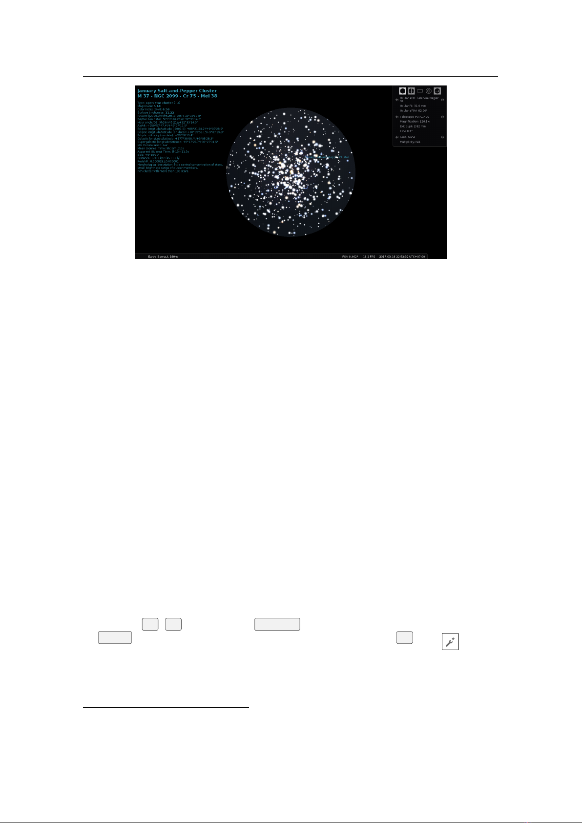
228 Chapter 16. Stellarium at the Telescope
Figure 16.5: The CCD sensor popup menu of the Oculars plugin.
Figure 16.6: Setting rotation of CCD sensor in the popup menu.
Figure 16.7: A rotated CCD sensor frame of the Oculars plugin.
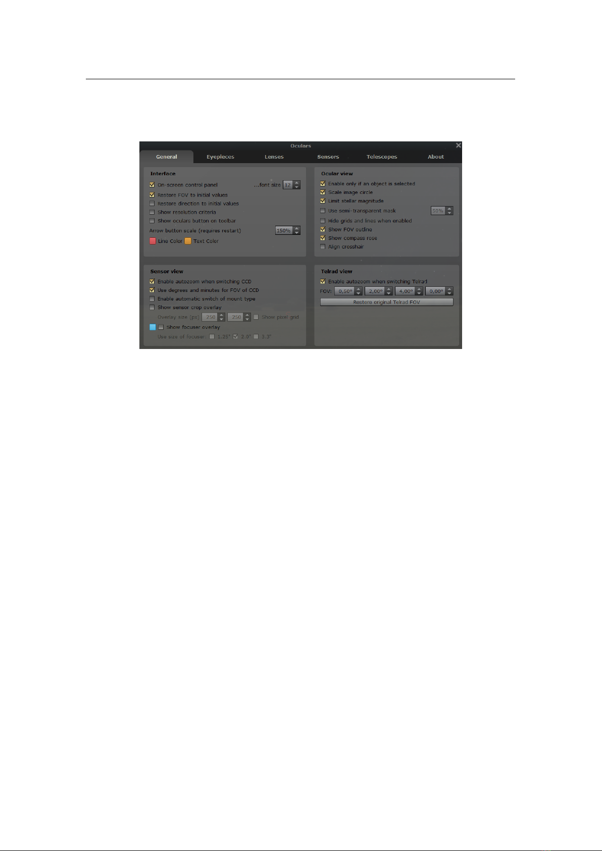
16.1 Oculars Plugin 229
Figure 16.8: The M37 cluster through a Celestron 15x70 binocular.
Figure 16.9: The M37 cluster through a Celestron 80 mm EDF with Explore Scientific 14 mm
eyepiece.
Figure 16.10: The M37 cluster through a Celestron C1400 with Tele Vue Nagler 31 mm eyepiece.

230 Chapter 16. Stellarium at the Telescope
telescope to be selected. Also notice that when your mouse cursor is very near the right hand border of the
screen, the popup menu’s sub-menus display to the left, not the right.
16.1.1.1 Star Scales
As you know from section 4.4.1, the number and relative size of stars of various magnitudes can be adjusted
to your personal preferences in the view settings window to approximate the appearance of the stars as seen
by the naked eye. Some observers prefer to have a simulated ocular view with very small, or more, stars,
quite different from what Stellarium usually shows. The Oculars plugin therefore keeps two additional sets
of scaling values for ocular views and CCD views, which are activated automatically when you switch to
ocular or CCD view, and which are stored immediately and permanently in the plugin’s ocular.ini file.
1
16.1.2 Configuration
All configuration is done through the user interface in the application. To open the configuration dialog hit
the
Alt
+
O
key, or click the
configure
button on the plugin setup dialog (available in the
Plugins
tab of
Stellarium’s Configuration window (opened by pressing
F2
or the button in the left toolbar)), or the
rightmost button of the on-screen panel (if displayed in the top right corner of screen). There are six tabs in
the configuration dialog: General, Eyepieces, Lenses, Sensors, Telescopes, and About. The first five are the
ones we are interested in here.
General
The first option allows you to define the general behavior of the plugin. The options are grouped by areas of
usage: Interface, Ocular view, Sensor view and Telrad view (see figure 16.11).
Figure 16.11: General tab of the Oculars plugin configuration dialog.
Interface: this group of options allows to change behavior of the plugin in general.
On-screen control panel:
show an additional GUI panel in the top-right corner of the screen to
allow switching features of the plugin (in addition to the popup window).
Restore FOV to initial values and
Restore direction to initial values
options allow restoration field of view and direction of view,
resp., to the initial values at program start at the end of the plugin usage (e.g., when disabling
the view through CCD frame).
Show resolution criteria
compute and show Rayleigh criterion, Dawes’, Abbe’s and Sparrow’s
limits for combination of telescope, lens and eyepiece. In addition, this option will show visual
resolution for selected “setup”. This option may be very helpful for double star observers.
Show oculars button on toolbar
option allows to toggle visibility the plugin button on main toolbar.
Arrow button scale allows to change the size of the arrow buttons in the ocular GUI panel.
1
The appearance of stars may depend on various other factors: telescope type, ocular type, quality of optics, seeing,
. . . Such details with all combinations cannot meaningfully be stored, though. These values should allow a rapid toggle
on any single night.
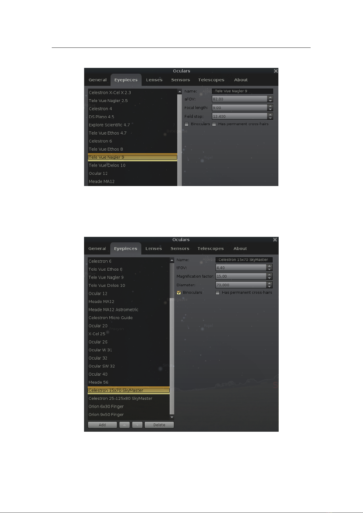
16.1 Oculars Plugin 231
Line Color Select color for ocular and sensor outlines and their labels.
Text Color
Select color for screen messages which are shown only when the on-screen control panel
is not shown.
Ocular view is a group of options that allows to change the plugin’s behavior in visual observation mode.
Enable only if an object is selected
– uncheck this option if you want to use the visual observation
mode when no object is selected.
Auto-limit stellar magnitude
sets the magnitude limitation for stars based on telescope diameter.
When disabled, the main program’s setting applies (see section 4.4.1). Note that two manual
limits for ocular view and main program are handled, and switching between ocular and main
view also switches those values.
Hide grids and lines when enabled
allows to hide grids and lines when you observe the sky through
the eyepiece and re-enables their visibility when leaving visual observation mode.
Scale image circle
option allows you to define whether or not to scale the images based on apparent
FOV. When deactivated, the image circle will fill your screen. In general, we recommend you
not select this, unless you have a need to, because it can really reduce the image size on the
screen. It can however be very useful in comparing two eyepieces. If you set this option, the
on-screen image will be scaled based on the eyepieces and telescopes you define. See section
16.1.3 for information on what scaling means, and why you might want to use it.
Use semi-transparent mask
uncheck this option if you want to see visible field of view as in real
telescope. You may define level of transparency for mask.
Hide grids and lines when enabled
allows to hide grids and lines when you observe the sky through
the eyepiece and re-enables their visibility when leaving visual observation mode.
Show FOV outline option enables drawing the border of the eyepiece’s FOV and it may be helpful
in combination with a semi-transparent mask.
Show compass rose
option enables drawing cardinal directions in the equatorial coordinate system.
Align crosshair
option enables alignment of the cross-hair according to the equatorial coordinate
system.
Sensor view
is group of options allows to change behavior of the plugin for photographic observations
mode.
Enable autozoom when switching CCD
Use degrees and minutes for FOV of CCD
– for many cases the use of decimal degrees for the
value of the field of view is not comfortable, and this option allows to use the more human
readable format for FOV.
Use horizontal coordinates instead of equatorial (J2000.0) coordinates in the top left frame cor-
ner.
Show max exposure time for moving objects
For solar system objects, the top right edge can in-
dicate the maximum exposure time so that the object moves less than a pixel against the
stars.
Enable automatic switch of mount type
allows to store the CCD frame orientation when the type
of telescope mount is changed.
Show sensor crop overlay
toggles drawing a crop box within the CCD frame. In addition, a pixel
grid can be drawn within the crop overlay especially for astrophotographers.
Show focuser overlay
allows drawing a circle which represents the telescope’s focuser. We added
sizes of 3 common modern focusers to allow users to check the visible aberrations in the FOV
of the telescope.
Telrad view is a group of options which allows to change behavior of the plugin for Telrad mode.
Enable autozoom when switching Telrad
option allows you to define whether or not to zoom the
field of view to twice the size of the Telrad circles.
FOV:
If you don’t use the original Telrad but a similar device, you may define up to 4 circles to show
its specific FOV in the sky.
Eyepieces
This is the tab used to enter your own eyepieces (see figures 16.12 and 16.13). By default, a few sample ones
have been added; feel free to delete those once you’ve entered your own.
The fields on this tab are:
Name
– a free-text description of the eye piece. You could modify this to match your personal descriptions
of eyepieces.
aFOV – apparent field of view in degrees.
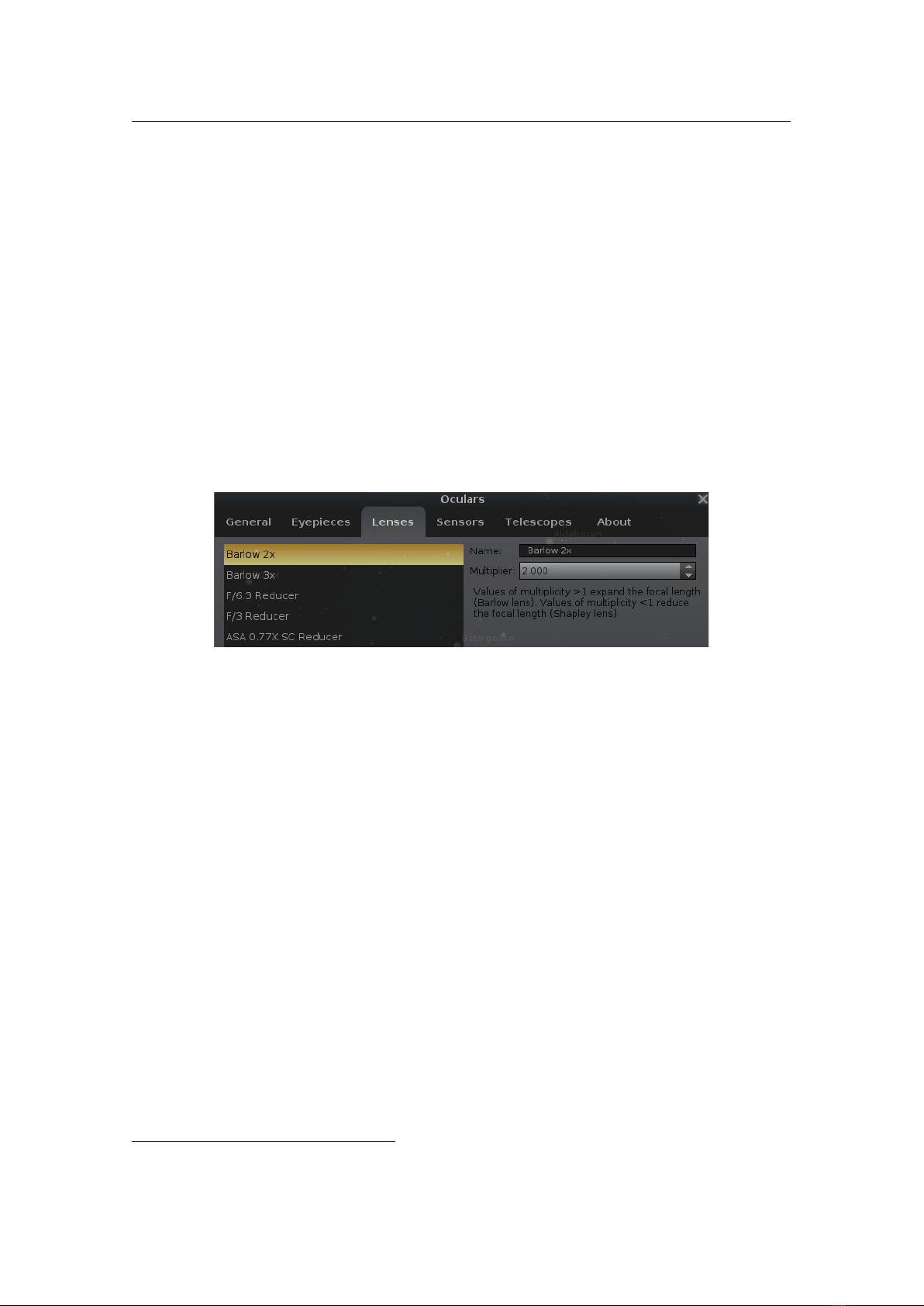
232 Chapter 16. Stellarium at the Telescope
Figure 16.12: Eyepieces tab of Oculars plugin configuration dialog.
Figure 16.13: Eyepieces tab of Oculars plugin configuration dialog (settings for binocular).
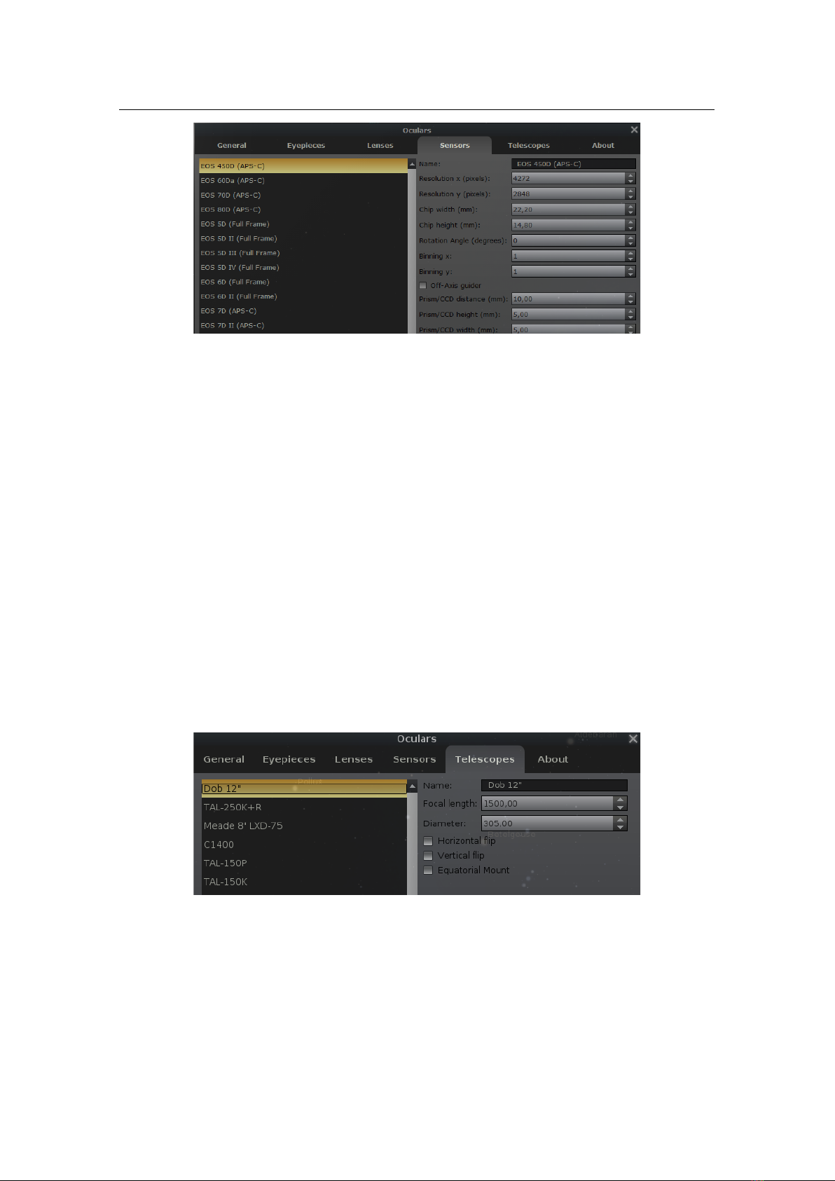
16.1 Oculars Plugin 233
Focal Length – eyepiece focal length in mm.
Field Stop
– the field stop of the eyepiece in
mm
. This is used to calculate the true field of view of an
eyepiece. If you do not know what it is just leave it the default zero. Not all manufacturers provide
this value; Tele Vue is one that does.
Binoculars
– selecting this checkbox tells the system that this eyepiece is binoculars or finders; this means
that this eyepiece can be used without defining a telescope.
Has permanent cross-hairs
– selecting this checkbox tells the system that this eyepiece or binocular (finder)
has also simple cross-hairs
2
.
When Binoculars are described, the relevant fields change to
tFOV
– true field of view in degrees. The true field of view can be given as meters at 1000 m. The
approximate conversion of this to degrees is to divide by 17.5. Thus, 87 m at 1000 m
= (8717.5)
°
≈ 5
°.
Magnification factor – the magnification of the binocular.
Diameter – the diameter of the binocular objective in mm.
For binoculars, we’re computed a few important factors in additional to the exit pupil
3
(these factors are
visible in an on-screen control panel):
Relative Brightness.
This is the square of the diameter of the exit pupil. For example, for a 10x50 binocular,
the exit pupil is 5
mm
and relative brightness is
(5010)
2
= 5
2
= 25
. However, the calculation for
a 20x100 binocular, through which a great deal more can be seen, gives exactly the same relative
brightness:
(10020)
2
= 5
2
= 25
, so this is an inadequate rating to use for astronomical binoculars.
Relative brightness is a number used to compare the brightness of binoculars of similar magnification.
The larger the relative brightness number, the brighter the image.
Twilight Factor
(Twilight Index or Twilight Performance Factor). This was used by Carl Zeiss Interna-
tional as an indication of the distance at which comparable detail would be seen in different binoculars.
It’s calculated by finding the square root of the product of the magnification and aperture. For the two
binoculars above, the calculations are:
(10∗ 50)=
(500)= 22.36
(20∗ 100)=
(2000)= 44.72
In this instance, the larger binocular has an index that is double that of the smaller binocular. Twilight
factor is a number used to compare the effectiveness of binoculars used in low light. The larger the
twilight factor, the more detail you can see in low light.
Bishop Index
(or Visibility Factor). This is due to Roy Bishop (Bishop, 2002) and is evaluated simply by
multiplying the magnification by the aperture in mm. For our two binocular above, we obtain:
10∗ 50 = 500
20∗ 100 = 2000
The larger binocular has a visibility factor four times greater than the smaller one.
Adler Index
(or Astro Index). This is due to Alan Adler (Adler, 2002) and is evaluated as the product of
the magnification and the square root of the aperture in
mm
. For our two binocular above, we obtain:
10∗
√
50 = 10∗ 7.1 = 71
20∗
√
100 = 20∗ 10 = 200
This gives the larger binocular an Astro Index of 2.8x the smaller one. At the moment this is the
best index to comparison of astronomical binoculars (of course for the simplest indexes, because
others have tried to expand on these by including the effect of coatings, baffles, and other aspects of
individual quality).
Lenses
This is the tab used to enter your own focal extender or reducer lenses (see figure 16.14). By default, a few
sample ones have been added; feel free to delete them once you’ve entered your own.
The fields on this tab are:
Name
– a free-text description of the lens. You could modify this to match your personal descriptions of
lenses.
2
The Oculars plugin supports eyepieces with reticle patterns – both special eyepieces are available in the default list
of eyepieces, and the option Has permanent cross-hairs is not related to those eyepieces.
3
The exit pupil diameter is calculated by dividing the aperture by the magnification.

234 Chapter 16. Stellarium at the Telescope
Figure 16.14: Lenses tab of Oculars plugin configuration dialog.
Multiplier
– a factor larger than 1 expands the focal length, and lenses with this type are named Barlow
lens; a factor less than 1 reduces the focal length, and lenses with this type are named Shapley lens or
focus reducer.
Sensors
This tab allows you to define sensors for any camera you may have (see figure 16.15). When defined and
selected, this will draw a red bounding rectangle in the center of the eye piece view, showing what the CCD
will capture. Because of the way floating point numbers are stored, sometimes you may see one of your
defined values change (for example from 2.2 to 2.19999) but this should not affect what you see.
Figure 16.15: Sensors tab of Oculars plugin configuration dialog.
The fields on this tab are:
Name – A free-text description of the sensor.
Resolution x – the width of the sensor in pixels.
Resolution y – the height of the sensor in pixels.
Chip width – the width of the sensor in mm.
Chip height – the height of the sensor in mm.
Rotation Angle – the rotation angle of the sensor, in degrees.
Binning x – the binning factor for the width of the sensor.
Binning y – the binning factor for the height of the sensor.
Off-Axis guider
– selecting this checkbox tells the system that this sensor has support an off-axis guider
also.
Prism/CCD distance
– distance between center of prism/CCD of Off-Axis Guider and optical axis of
telescope in mm.
Prism/CCD width – the width of the prism/CCD of Off-Axis Guider in mm.
Prism/CCD height – the height of the prism/CCD of Off-Axis Guider in mm.
Position Angle – the position angle of the prism/CCD of Off-Axis Guider, in degrees.
The resolution is easy to find: these are simply the image dimensions of a (non-binned) frame. The chip size
and pixel size may be more difficult, but the manual, or searching the Internet, should turn up these values.
For a “full-frame” DSLR, this should be close to 36x24
mm
, while APS-C should be around 22.5x15
mm
.
Some cameras may have unsquare pixels.
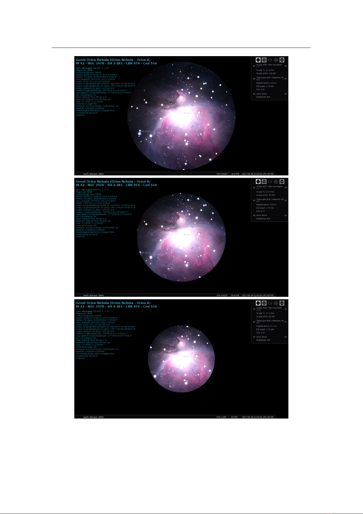
16.1 Oculars Plugin 235
Telescopes
This is the tab used to enter your own telescopes and photographic objectives (see fig. 16.16). The fields on
this tab are:
Figure 16.16: Telescopes tab of Oculars plugin configuration dialog.
Name – A free-text description of the telescope.
Focal Length – telescope focal length f in mm.
Diameter
– telescope diameter (aperture
∅
) in
mm
. If you add a photographic objective that does not
provide this information but provides a largest f stop like “100
mm
f/2.8”, you can estimate from
∅ = f s, where s = 2.8 and thus ∅ = 1002.8 = 35.7mm in this example.
Horizontal flip – if the view through this telescope should flip horizontally.
Vertical flip – if the view through this telescope should flip vertically.
Equatorial Mount – select it if this telescope has an equatorial mount.
16.1.3 Scaling the eyepiece view
I (TR) would like to thank Al Nagler over at Tele Vue
4
for helping to set me straight on the topic of eyepieces.
They are a lot more complicated than you might think!
By default, the view drawn on your computer screen when the plugin is active fills the screen. That is,
there is a circle drawn to represent the view through the eyepiece, and this circle will fill the screen. For
general use, this is what most people would want. There will be times that it’s not.
If you are going to be observing any deep space object, it can be very important to choose the best
eyepiece for that object. You will typically want an eyepiece that will magnify the object as much as possible,
while showing all of the object in the eyepiece view. Getting this can be tricky, especially if you do not like
changing eyepieces at the telescope. Or maybe you want to understand why one type of telescope may be
better than another type for observing what you are interested in. This is where you will want to scale the
image on screen based on your eyepiece.
Different eyepieces generally have a different apparent field of view (aFOV). An easy way to think about
this is: the larger the aFOV, the bigger the picture you see in the eyepiece. Older types of eyepiece (some
types still built and in wide use today have been constructed in the 19th century) generally have their aFOV
in the
50
° range. Today, there are massive eyepieces available with
82
°, and recently even
100
° aFOV! These
eyepieces are huge, as they require a lot of very special glass to achieve their incredible fields of view. An
eyepiece of the same focal length with a
100
° aFOV will produce an image through the eyepiece that is twice
as wide as one produced by a 50° eyepiece.
Different telescopes, with an eyepiece of a given aFOV, will also produce a different true field of view.
This is the actual size of the piece of sky that you see through the eyepiece. Getting these two “just right”
can be very important. It’s easy to assume that you want the biggest telescope you can get, with the eyepiece
that gives you the highest magnification. This is never true in reality. Depending on where you live, and
especially what you like to look at, a 100-120
mm
quality refractor with a wide aFOV eyepiece may very
well be better than a large SCT with the same eyepiece. This is something I learned the hard way.
So how does scaling the eyepiece view help? The plugin will find the eyepiece you have with the largest
aFOV. This aFOV becomes
100%
of the computer screen diameter. Then, any other eyepiece will have its
aFOV compared, and the view on screen will be scaled down accordingly. These
100
° aFOV eyepieces
makes the math here easy. If you have one, then when that eyepiece is used, the circle that represents the
view through the eyepiece will take up
100%
of the screen diameter. Next, if you select an eyepiece with an
4
https://www.televue.com/

236 Chapter 16. Stellarium at the Telescope
82
° aFOV, its view will be scaled to
82%
of the screen, and a
62
° aFOV eyepiece will be scaled to
62%
of
the screen.
Example in action
This is easier to understand in action, so let us look at an example that uses three eyepieces all with the same
17
mm
focal length, so they all produce the same level of magnification (well, one has an 17.3
mm
focal
length, but its magnification is nearly identical) and see how the view changes. These example all use a
Celestron C8 8" SCT telescope, and the target is the Great Orion Nebula.
We can see from the images in fig. 16.17 that the target is all three images is the same size. The
100
°
image fills the screen, the
82
° is smaller, and the
62
° is smallest yet, filling
62%
of the computer screen.
Note that in each image, the field of view that you see changes. The larger the aFOV, the more you can see
of the sky. So in this example, if you had an 8" telescope, you would want to use the 17
mm 100
° Ethos
eyepiece to see as much of the nebula as possible.

16.1 Oculars Plugin 237
Figure 16.17: Comparing apparent fields of view of (top) a 17
mm
Tele Vue Ethos eyepiece with an
aFOV of
100
°. Magnification is
119.5×
. (center) a 17
mm
Tele Vue Nagler eyepiece with an aFOV
of
82
°. Magnification is
119.5×
. (bottom) a 17.3
mm
Tele Vue Delos eyepiece with an aFOV of
62°. Magnification is 117.5×.

238 Chapter 16. Stellarium at the Telescope
16.2 TelescopeControl Plugin
This plugin provides a simple control mechanism for motorized telescope mounts. The user selects an object
(i.e. by clicking on something – a planet, a star etc.) and presses the telescope go-to key, and the telescope
will be guided to the object.
Multiple telescopes may be controlled simultaneously.
WARNING
Stellarium cannot prevent your telescope from being pointed at the Sun. It is up to you to ensure proper
filtering and safety measures are applied!
Never point your telescope at the Sun without a proper solar filter installed. The powerful light amplified
by the telescope WILL cause irreversible damage to your eyes and/or your equipment.
Even if you don’t do it deliberately, a slew during daylight hours may cause your telescope to point
at the sun on its way to the given destination, so it is strongly recommended to avoid using the telescope
control feature before sunset without appropriate protection.
16.2.1 Abilities and limita tions
This plug-in allows Stellarium to send ’slew’ (’go to’) commands to the device and to receive its current
position. There are some scopes which additionally support ’sync’ commands to be received in order to
update the internal pointing model of the mount. Some scopes also have the ability to abort a previous
slew command. However, users should always be aware of the possibility for mount collisions and similar
situations. You should always make sure that a slew does not cause parts of the telescope to collide with the
environment or mount itself.
Currently this plug-in does not allow satellite tracking unless the controlled telescope is an RTS2 system
(see section 16.2.6), and is not very suitable for lunar or planetary observations. Many mounts can be set to a
’lunar’ tracking speed, you may prefer this.
Some users are running Stellarium on little, low-power “Telescope computers” connected to their
powerful indoor PCs via RemoteDesktop or similar setups. Keep in mind that Stellarium is a graphics-heavy
program that may challenge the outdoor computer’s graphics subsystem or network. See framerate intent
settings on page 26 for optimizing your screen refresh rates. Better, run Stellarium on your indoor system
and use INDI or ASCOM network protocols.
16.2.2 Using this plug-in
Here are two general ways to control a device with this plug-in, depending on the situation:
DIRECT CONNECTION
A device supported by the plug-in is connected with a cable to the computer
running Stellarium
INDIRECT CONNECTION
local
A device is connected to the same computer but it is driven by a stand-alone telescope server
program or a third-party application that can ’talk’ to Stellarium;
remote
A device is connected to a remote computer and the software that drives it can ’talk’ to
Stellarium over the network; this software can be either one of Stellarium’s stand-alone telescope
servers, or a third party application.
Most older telescopes use cables that connect to a serial port (RS-232), the newer ones use USB (Universal
Serial Bus). On Linux and Max OS X, both cases are handled identically by the plug-in. On Windows,
a USB connection may require a ’virtual serial port’ software, if it is not supplied with the cable or the
telescope. Such a software creates a virtual (’fake’) COM port that corresponds to the real USB port so it can
be used by the plug-in. On all three platforms, if the computer has no ’classic’ serial ports and the telescope
can connect only to a serial port, a serial-to-USB (RS-232-to-USB) adapter may be necessary.
Telescope set-up (setting geographical coordinates, performing alignment, etc.) should be done before
connecting the telescope to Stellarium.
16.2.3 Main window (’Telescopes’)
The plug-in’s main window can be opened:
•
By pressing the
configure
button for the plug-in in the
Plugins
tab of Stellarium’s Configuration
window (opened by pressing
F2
or the
button in the left toolbar).
•
By pressing the
Configure telescopes...
button in the
Slew to
window (opened by pressing
Ctrl
+
0
or the respective button on the bottom toolbar).
The
Telescopes
tab displays a list of the telescope connections that have been set up:
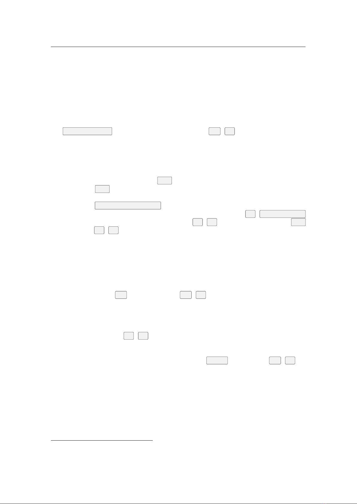
16.2 TelescopeControl Plugin 239
•
The number (#) column shows the number used to control this telescope. For example, for slewing
telescope #2, the shortcut is
Ctrl
+
2
.
•
The Status column indicates if this connection is currently active or not. Unfortunately, there are some
cases in which ’Connected’ is displayed when no working connection exists.
•
The Type field indicates what kind of connection this is:
virtual means a virtual telescope (test mode).
direct, Stellarium means a DIRECT connection to the telescope (see above).
local, external means an INDIRECT connection to a program running on the same computer.
local, ASCOM
means an INDIRECT connection to a ASCOM driver running on the same computer.
remote, unknown means an INDIRECT connection over a network to a remote machine.
remote, RTS2 means an INDIRECT connection over a network to an RTS2 server.
remote, INDI means an INDIRECT connection over a network to an INDI server.
To set up a new telescope connection, press the
Add
button. To modify the configuration of an existing
connection, select it in the list and press the
Configure
button. In both cases, a telescope connection
configuration window will open.
16.2.4 Telescope configuration window
Connection type
The topmost field represents the choice between the types of connections (see section 16.2.2): Telescope
controlled by:
Stellarium, directly (serial or network)
is the DIRECT case. LX200-compatible mounts can be connected
either through a serial port or, over a TCP/IP network (see Device settings). v 26.3
External software or a remote computer is an INDIRECT case
RTS2 Telescope is another INDIRECT case
INDI is another INDIRECT case
ASCOM is another INDIRECT case
Nothing, just simulate one (a moving reticle) is a virtual telescope (no connection)
Telescope properties
Name is the label that will be displayed on the screen next to the telescope reticle.
Connection delay
If the movement of the telescope reticle on the screen is uneven, you can try increasing
or decreasing this value.
Coordinate system
Some Celestron telescopes have had their firmware updated and now interpret the
coordinates they receive as coordinates that use the equinox of the date (EOD, also known as JNow),
making necessary this setting. With ASCOM telescopes it’s also possible to use this setting to override
the default device preference.
Start/connect at startup
Check this option if you want Stellarium to attempt to connect to the telescope
immediately after it starts. Otherwise, to start the telescope, you need to open the main window, select
that telescope and press the
Start/Connect
button.
Device settings
This section is active only for DIRECT connections (see above).
v 26.3
Connection
selects Serial port or, for LX200-compatible mounts, Network (TCP) – the LX200 protocol
spoken directly over TCP/IP. With Network (TCP) the Serial port field is replaced by Host and Port
(the telescope’s network address and TCP port).
Serial port sets the serial port used by the telescope. A pop-up box suggests some default values:
•
On Windows, serial ports COM1 to COM10
•
On Linux, serial ports are labelled
/dev/ttyS0
to
/dev/ttyS3
and USB ports
/dev/ttyUSB0
to
/dev/ttyUSB3
. Make sure you have read/write access to the
tty
device. Depending on
your flavour of Linux, this may e.g. require some group membership.
•
On macOS, the list is empty as it names its ports in a peculiar way. If you are using a USB
cable, the default serial port of your telescope most probably is not in the list of suggestions. To
list all valid serial port names in macOS, open a terminal and type:
ls / dev /*
This will list all devices, the full name of your serial port should be somewhere in the list (for
example, /dev/cu.usbserial-FTDFZVMK).
Device model : see 16.2.5 Supported devices.

240 Chapter 16. Stellarium at the Telescope
Connection settings
Both fields here refer to INDIRECT connections, which implies communication over a network (TCP/IP).
Host
can be either a host name or an IPv4 address such as ’127.0.0.1’. The default value of ’localhost’
means ’this computer’.
Modifying the default host name value makes sense only if you are attempting a remote connection
over a network. In this case, it should be the name or IP address of the computer that runs a program
that runs the telescope.
Port
refers to the TCP port used for communication. The default value depends on the telescope number
and ranges between 10001 and 10009.
RTS2 settings
(see also 16.2.6) You will need access to an RTS2 HTTPD server through HTTP/JSON calls. Please see
RTS2 documentation (man rts2-httpd) for details. You will as well need username and password for HTTPD.
Please be aware that in order to move the telescope, your user must have the telescope in the list of allowed
devices in the database. Please see man rts2-user for details on how to manipulate RTS2 users.
URL
points to RTS2 HTTPD. Can include anything a URL can have - port (:8889) and prefix path for RTS2
access.
Username username used for login to RTS2 HTTPD.
Password password for login to RTS2 HTTPD.
INDI settings
(see also 16.2.7) You will need access to an INDI server through a TCP/IP connection. Please see INDI
documentation for details. You will need to select the correct INDI device to manage it.
ASCOM settings
You can choose an ASCOM telescope driver installed in your system using the ASCOM chooser. Additionally
you can choose how Stellarium is determining the coordinate system used to communicate with the ASCOM
mount. For more information, please see 16.2.8.
User Interface Settings: Field of view indicators
A series of circles representing different fields of view can be added around the telescope marker. This is a
relic from the times before the Oculars plug-in (see 16.1) existed.
Activate the ’Use field of view indicators’ option, then enter a list of values separated with commas in
the field below. The values are interpreted as degrees of arc.
These marks can be used in combination with a virtual telescope to display a moving reticle with the
Telrad circles.
16.2.4.1 ’Slew telescope to’ window
The
Slew telescope to
window can be opened by pressing
Ctrl
+
0
or the respective button in the bottom
toolbar.
It contains two fields for entering celestial coordinates, selectors for the preferred format (Hours-Minutes-
Seconds, Degrees-Minutes-Seconds, or Decimal degrees), a drop-down list and two buttons.
The drop-down list contains the names of the currently connected devices. If no devices are connected,
it will remain empty, and the
Slew
button will be disabled.
Pressing the
Slew
button slews the selected device to the selected set of coordinates. See the section
about keyboard commands below for other ways of controlling the device.
Pressing the
Configure telescopes. . .
button opens the main window of the plug-in.
TIP: Inside the ’Slew’ window, underlined letters indicate that pressing
Alt
+
underlined letter
can be
used instead of clicking. For example, pressing
Alt
+
S
is equivalent to clicking the
Slew
button, pressing
Alt
+
E
switches to decimal degree format, etc.
16.2.4.2 Sending commands
Once a telescope is successfully started/connected, Stellarium displays a telescope reticle labelled with the
telescope’s name on its current position in the sky. The reticle is an object like every other in Stellarium - it
can be selected with the mouse, it can be tracked and it appears as an object in the ’Search’ window.
To point a device to an object: Select an object (e.g. a star) and press the number of the device while
holding down the
Ctrl
key. (For example,
Ctrl
+
1
for telescope #1.) This will move the telescope to
the selected object. Note that most telescopes can only execute a single command to move to that object’s
position, but if the telescope is an RTS2 telescope, you can even track a satellite (if the mount then is fast
enough to support it).
5
5
Actually, the TLE orbital elements of the selected satellite are transmitted to RTS2, which does then compute the

16.2 TelescopeControl Plugin 241
To point a device to the center of the view: Press the number of the device while holding down the Alt
key. (For example,
Alt
+
1
for telescope #1.) This will slew the device to the point in the center of the
current view. (If you move the view after issuing the command, the target won’t change unless you issue
another command.)
To point a device to a given set of coordinates: Use the
Slew to
window (press
Ctrl
+
0
).
16.2.5 Supported devices
16.2.5.1 Directly connected telescopes
All devices listed in the ’Device model’ list are convenience definitions using one of the two built-in
interfaces: the Meade LX200 (the Meade Autostar controller) interface and the Celestron NexStar interface.
The device list contains the following:
Celestron NexStar (compatible) Any device using the NexStar interface.
Losmandy G-11
A computerized telescope mount made by Losmandy (Meade LX-200/Autostar interface).
Meade Autostar compatible Any device using the LX-200/Autostar interface.
Meade ETX-70 (#494 Autostar, #506 CCS)
The Meade ETX-70 telescope with the #494 Autostar con-
troller and the #506 Connector Cable Set. According to the tester, it is a bit slow, so its default setting
of ’Connection delay’ is 1.5 seconds instead of 0.5 seconds.
Meade LX200 (compatible) Any device using the LX-200/Autostar interface.
Sky-Watcher SynScan AZ mount
The Sky-Watcher SynScan AZ GoTo mount is used in a number of
telescopes.
Sky-Watcher SynScan (version 3 or later)
SynScan is also the name of the hand controller used in other
Sky-Watcher GoTo mounts, and it seems that any mount that uses a SynScan controller version 3.0 or
greater is supported by the plug-in, as it uses the NexStar protocol.
Wildcard Innovations Argo Navis (Meade mode)
Argo Navis is a ’Digital Telescope Computer’ by Wild-
card Innovations. It is an advanced digital setting circle that turns an ordinary telescope (for example,
a dobsonian) into a ’Push To” telescope (a telescope that uses a computer to find targets and human
power to move the telescope itself). Just don’t forget to set it to Meade compatibility mode and set the
baud rate to 9600B1.
16.2.5.2 RTS2 telescopes
Setting up a robotic telescope and dome control system with RTS2 is beyond the scope of this handbook, but
see section 16.2.6 for a few notes to be able to connect and command the telescope with Stellarium. Please
refer to the RTS2 Web pages
6
for further details.
Please be aware that some RTS2 usernames might have only read-only access. If this is case for your
username, the telescope marker will be painted red (or
color_telescope_readonly
from Stellarium’s
settings file).
16.2.5.3 INDI telescopes
Setting up a robotic telescope and dome control system with INDI is beyond the scope of this handbook, but
see section 16.2.7 for a few notes to be able to connect and command the telescope with Stellarium. Please
refer to the INDI web pages
7
for further details.
16.2.5.4 ASCOM telescopes
ASCOM specific settings can be configured when a ASCOM telescope was selected. Please see section 16.2.8
for further information about configuration possibilities.
16.2.5.5 Virtual telescope
If you want to test this plug-in without an actual device connected to the computer, choose “Nothing, just
simulate one (a moving reticle)” in the
Telescope controlled by:
field. It will show a telescope reticle that
will react in the same way as the reticle of a real telescope controlled by the plug-in. See the section above
about field of view indicators for a possible practical application (emulating ’Telrad’ circles).
16.2.6 RTS2
RTS2, the Remote Telescope System 2, is a complete robotic observatory control system for Linux by Petr
Kubánek, who kindly provided the plugin code to make RTS2 interoperate with Stellarium. We cannot give a
full manual or any further support for RTS2 here, please refer to its website
8
for complete instructions about
satellite position itself.
6
https://rts2.org/
7
https://indilib.org
8
https://rts2.org

242 Chapter 16. Stellarium at the Telescope
dome control, cameras, filter wheels, weather sensors, etc. A few notes may be useful for beginners, though.
RTS2’s central piece is a daemon. Start the system:
sudo service rts2 start
RTS2’s main control screen is text-based, rts2-mon. For a quick check, switch on the system using
F9
.
Telescope
T0
is a dummy telescope which you can select and operate with commands like
move 120 35
(this moves to RA=120°=8h, DEC=35°, but only when this position is above your horizon).
Stellarium’s Telescope plugin can communicate with RTS2 using the RTS2 web interface. You must
run rts2-httpd for this, which may require the right permissions to write the lock files in
/var/run
. This
program requires that a database has been created as described in the file
RUN
in RTS2’s source directory and
on the RTS2 website
9
. Also, you must create a ’user’ for RTS2. This is not a regular Linux account, but an
entry in the RTS2 database. Create a user with rts2-user -a <user>. You should use a password different
from your regular Linux password, as this will be transmitted in plain text between the computer running
Stellarium and the RTS2 control computer, and may also be written into Stellarium’s logfile. Then you can
enable device control for the respective user. If you want to send slew commands from Stellarium, make
sure to allow access to telescope
T0
. If not, Stellarium will be able to show the telescope marker, but you
will not be able to control the telescope. To enable control for existing users in the default stars database,
psql stars
update users set allow ed_de vices = ’* ’;
In case you cannot properly connect to the RTS2 telescope or cannot send slew commands, check
Stellarium’s logfile log.txt for some diagnostic messages.
RTS2 is the only type of telescope supported by Stellarium which can autonomously track satellites.
Tracking accuracy fully depends on Stellarium’s TLE satellite elements being up-to-date (see section 14.8)
and the accuracy of your RTS2 installation.
16.2.7 INDI
INDI, the Instrument Neutral Distributed Interface, is a distributed control system (DCS) protocol to enable
control, data acquisition and exchange among hardware devices and software front ends, emphasizing
astronomical instrumentation
10
.
INDI client (v1.6.0) has been incorporated into Stellarium’s Telescope Control plugin by Alessandro
Siniscalchi to allow Stellarium to communicate with INDI hardware drivers via INDI server. INDI server is
a hub that sits between drivers and clients. It reroutes traffic for control and data across distributed networks.
Each device or client in the network is a node and may communicate with other nodes whenever desired.
The server supports broadcasting, chaining, and marshalling of data.
Stellarium only supports INDI mounts (no other INDI devices), and you will need to select the correct
INDI device to manage it at the stage of configuration of telescope. For this purpose the plug-in has a tool
to getting the list of connected devices from the INDI server (when the server is working!). Please define
hostname and port
11
in the “INDI Settings” block, press
Refresh devices
and select the required device in
the list “Devices”.
List of telescope types supported by INDI
12
:
•
Meade Autostar
•
Meade LX200 (Classic/GPS/16)
•
Celestron NexStar
•
Celestron NexStar Evolution
•
Orion Synscan Telescope
•
EQ-6 MCU Update
•
HEQ-5 MCU Update
•
LittleFoot Vpower
•
LittleFoot Elegance Photo
•
Astro-Electronic FS-2
•
EQMod
9
https://rts2.org/faq.html
10
https://en.wikipedia.org/wiki/Instrument_Neutral_Distributed_Interface
11
The Internet Assigned Numbers Authority (IANA) has assigned to INDI the Transmission Control Protocol and
User Datagram Protocol (TCP/UDP) port 7624.
12
https://indilib.org/devices/telescopes/all.html

16.2 TelescopeControl Plugin 243
•
Pulsar2
•
SkySensor2000PC
•
Takahashi Temma
•
10 Micron
•
Losmandy Gemini
•
Astrophysics
•
Skywatcher Virtuoso (Alt/Az)
•
IOptron IEQPro/CEM60
•
IOptron ZEQ25/SmartEQ
•
IOptron GotoNova Upgrade Kit 8400
16.2.8 ASCOM 7 (Windows only)
ASCOM is probably the most widely used way how to communicate with telescopes, mounts and other
astronomy equipment on Microsoft Windows operating systems. The ASCOM platform aims to decouple
device dependent specifics by introducing a common standard for communication between device drivers
and applications. Almost every telescope mount comes with an ASCOM driver and most of the astronomy
software and tools can communicate with ASCOM compatible devices.
The ASCOM telescope support has been added to Stellarium’s Telescope Control plugin by Gion Kunz
in version 0.19.3.
13
Note that in order for Stellarium to communicate with your ASCOM compatible mount, you will need
to have the ASCOM platform installed on your Windows machine (version 7 or higher
14
; On Windows 11
for ARM64, ASCOM platform 7.1.2 or later is required.). Also, the ASCOM driver of your telescope mount
needs to be installed before you can start using the telescope in Stellarium.
Important: Most modern ASCOM drivers are written to run in 32bit and 64bit mode (any) and therefore
are compatible with the 64bit and 32bit version of Stellarium. However, if you happen to have a 32bit or
64bit only driver for your telescope mount, you will also need to install the respective Stellarium version.
In order to use your ASCOM telescope you need to select the correct device in the ASCOM chooser by
clicking the button
Choose ASCOM telescope
. The selected device is shown below that button.
By default, Stellarium is trying to ask the ASCOM driver in order to determine if JNow or J2000
coordinates should be used for communicating with the mount. If you’d like to override this behavior and
tell the ASCOM telescope to communicate in the coordinate system configured in the section Telescope
properties, you can switch the radio button
Let ASCOM device decide
to
Use Stellarium settings
in the
ASCOM settings of the Configure Telescope dialog.
16.2.9 StellariumScope
StellariumScope is a free add-on that enables you to control your ASCOM enabled telescope with Stellarium.
Note that Stellarium supports ASCOM telescopes natively since version 0.19.3. There’s no need to use
StellariumScope in order to use your ASCOM telescopes with Stellarium anymore. We are encouraging our
users to use the native ASCOM option unless they need particular features of StellariumScope.
The original StellariumScope program was designed and implemented by Scott of ByteArts but is no
longer available. It is now maintained by and available for download from Welsh Dragon Computing
15
.
Features
•
Provides an interface between Stellarium and ASCOM telescope drivers.
•
Provides the ability to both “Sync” and “Slew” the telescope. It’s also possible to issue a stop/cancel
command from Stellarium.
•
You can easily host Stellarium on one computer linked to another control computer that hosts the
telescope driver.
•
The installation program will automatically install the documentation, but the link to the documentation
is provided by the developer
16
so you can read it before installation.
13
Unfortunately ASCOM version 6 seems to be incompatible with Qt6. After numerous error reports we had to
disable ASCOM support on Qt6-based builds of version 24.3-24.4. However, preliminary tests showed that ASCOM 7
may work again, so this way of connection is back. Without proper instruments, the maintainers depend on your feedback,
though. If you depend on ASCOM support, please update to ASCOM version 7, or use a Qt5-based build of the same
version.
14
https://ascom-standards.org/Downloads/Index.htm
15
https://welshdragoncomputing.ca/x/index.php/home/stellariumscope/about-stellariumscope
16
StellariumScope User’s Guide —
https://welshdragoncomputing.ca/x/st/misc/stellariumscope_

244 Chapter 16. Stellarium at the Telescope
Use this application (like all software that controls your mount) with supervision of your mount’s
movements.
16.2.10 Other telescope servers and Stellarium
Other developers have also been busy creating hard- and software often involving Arduino or Raspberry
Pi boards which can control GOTO or PUSHTO (manually driven but position-aware, usually Dobsonian)
telescopes and are ultimately controlled from Stellarium. Those are not related nor authored by the Stel-
larium team, so while we welcome such development (esp. open-sourced) in general, we cannot provide
documentation nor any support.
A few examples:
iTelescope http://simonbox.info/index.php/astronomy/93-raspberry-pi-itelescope
node-telescope-server https://www.npmjs.com/package/node-telescope-server
OnStep https://groups.io/g/onstep
One anonymous user sent a troubleshooting solution when connecting Stellarium to the Celestron
NexRemote software:
One tricky Window XP issue I fixed was that my older laptop would transiently lose connection
with Stellarium although the status would still be “Connected” and all looked normal. [. . . ]
I boosted the NexRemote.exe process in Windows XP to High under Set Priority under the
Windows Task Manager via
Ctrl
+
Alt
+
Del
.
All slews now proceed normally. Problem went away.
17
16.2.10.1 Stellarium Telescope Protocol
In the early days of Stellarium, telescope control required standalone server programs. These were later
integrated in the plugin. However, there are situations where external control servers are still useful, e.g.
when they are running on some tiny telescope computer while the user sits in the warm control room in front
of the powerful PC running Stellarium. For you DIYers out there, figure 16.18 shows the original protocol.
user_guide.2016.03.05.pdf
17
https://sourceforge.net/p/stellarium/discussion/278769/thread/16e4c054/?limit=25#8ffa

16.2 TelescopeControl Plugin 245
/*
Author and Copyright of this file and of the stellarium telescope library:
Johannes Gajdosik, 2006
*/
Stellarium Telescope Protocol version 1.0
The Stellarium Telescope Protocol works on top of TCP/IP.
The client is the stellarium program (or any similar program),
the server is called "telescope server" and controls the telescope.
Depending on the implementation the server may handle one or many
simultaneous clients. The reference server implementation accepts
an unlimited number of simultaneous clients.
The protocol is message based: both server and client may
spontaneousely send messages as often as they want.
When the server looses control of the telescope he should
actively close the connection to all clients.
The first two bytes of any message describes the total
length of that message in bytes (including the first 2 bytes).
The next 2 bytes of any message describe the type of this message.
The byte order for all kind of integers is always
"least significiant byte first".
-----------------------
server->client:
MessageCurrentPosition (type = 0):
LENGTH (2 bytes,integer): length of the message
TYPE (2 bytes,integer): 0
TIME (8 bytes,integer): current time on the server computer in microseconds
since 1970.01.01 UT. Currently unused.
RA (4 bytes,unsigned integer): right ascension of the telescope (J2000)
a value of 0x100000000 = 0x0 means 24h=0h,
a value of 0x80000000 means 12h
DEC (4 bytes,signed integer): declination of the telescope (J2000)
a value of -0x40000000 means -90degrees,
a value of 0x0 means 0degrees,
a value of 0x40000000 means 90degrees
STATUS (4 bytes,signed integer): status of the telescope, currently unused.
status=0 means ok, status<0 means some error
---------------------
client->server:
MessageGoto (type =0)
LENGTH (2 bytes,integer): length of the message
TYPE (2 bytes,integer): 0
TIME (8 bytes,integer): current time on the client computer in microseconds
since 1970.01.01 UT. Currently unused.
RA (4 bytes,unsigned integer): right ascension of the telescope (J2000)
a value of 0x100000000 = 0x0 means 24h=0h,
a value of 0x80000000 means 12h
DEC (4 bytes,signed integer): declination of the telescope (J2000)
a value of -0x40000000 means -90degrees,
a value of 0x0 means 0degrees,
a value of 0x40000000 means 90degrees
Figure 16.18: The Stellarium Telescope Protocol, version 1.0

246 Chapter 16. Stellarium at the Telescope
16.3 Observability Plugin
This Plugin is activated with the button . It analyzes the observability of the selected object (or the
screen center, if no object is selected). The plugin can show the best epoch of the year (i.e., largest angular
separation from the Sun), the date range when the source is above the horizon at dark night, and the dates of
Acronychal and Cosmical rise/set. Ephemerides of the Solar-System objects and parallax effects are taken
into account.
Explanation of some parameters
Sun altitude at twilight
Any celestial object will be considered visible when the Sun is below this altitude.
The altitude at astronomical twilight ranges usually between -12 and -18 degrees. This parameter is
only used for the estimate of the range of observable epochs (see below).
Horizon altitude Minimum observable altitude (due to obstructions or just a limited telescope mount).
Acronychal/Cosmical/Heliacal rise/set
The days of Cosmical rise/set of an object are estimated as the
days when the object rises (or sets) together with the rise/set of the Sun. The exact dates of these
events depend on the Observer’s location. In contrast, the Acronychal rise (or set) happens when the
star rises/sets with the setting/rising of the Sun (i.e., opposite to the Sun). It is obvious that the source
is hardly observable (or not observable at all) in the dates between Cosmical set and Cosmical rise.
On the other hand, the dates around the Acronychal set and rise are those when the altitude of the
celestial object uses to be high when the Sun is well below the horizon (hence the object can be well
observed). The date of Heliacal rise is the first day of the year when a star becomes visible. It happens
when the star is close to the eastern horizon roughly before the end of the astronomical night (i.e., at
the astronomical twilight). In the following nights, the star will be visible during longer periods of
time, until it reaches its Heliacal set (i.e., the last night of the year when the star is still visible). At the
Heliacal set, the star sets roughly after the beginning of the astronomical night.
Largest Sun separation
Happens when the angular separation between the Sun and the celestial object
are maximum. In most cases, this is equivalent to say that the Equatorial longitudes of the Sun and
the object differ by 180 degrees, so the Sun is in opposition to the object. When an object is at its
maximum possible angular separation from the Sun (no matter if it is a planet or a star), it culminates
roughly at midnight, and on the darkest possible area of the Sky at that declination. Hence, that is the
’best’ night to observe a particular object.
Nights with source above horizon
The program computes the range of dates when the celestial object is
above the horizon at least during one moment of the night. By ’night’, the program considers the time
span when the Sun altitude is below that of the twilight (which can be set by the user; see above).
When the objects are fixed on the sky (or are exterior planets), the range of observable epochs for the
current year can have two possible forms: either a range from one date to another (e.g., 20 Jan to 15
Sep) or in two steps (from 1 Jan to a given date and from another date to 31 Dec). In the first case, the
first date (20 Jan in our example) shall be close to the so-called ’Heliacal rise of a star’ and the second
date (15 Sep in our example) shall be close to the ’Heliacal set’. In the second case (e.g., a range in
the form 1 Jan to 20 May and 21 Sep to 31 Dec), the first date (20 May in our example) would be
close to the Heliacal set and the second one (21 Sep in our example) to the Heliacal rise. More exact
equations to estimate the Heliacal rise/set of stars and planets (which will not depend on the mere
input of a twilight Sun elevation by the user) will be implemented in future versions of this plugin.
Full Moon
When the Moon is selected, the program can compute the exact closest dates of the Moon’s
opposition to the Sun.
Note on Terminology
The (sparse) literature on terminology about computing these Heliacal, Acronychal or Cosmic events seems
to disagree on which end of the night is to be computed. While all agree about Heliacal rises taking place in
the morning, Acronychal and Cosmic are sometimes applied in reverse order from those described here. In
case you use these data, make sure you keep this definition as well.
Author
This plugin has been contributed by Ivan Marti-Vidal (Onsala Space Observatory)
18
with some advice by
Alexander Wolf and Georg Zotti.
18
mailto:i.martividal@gmail.com
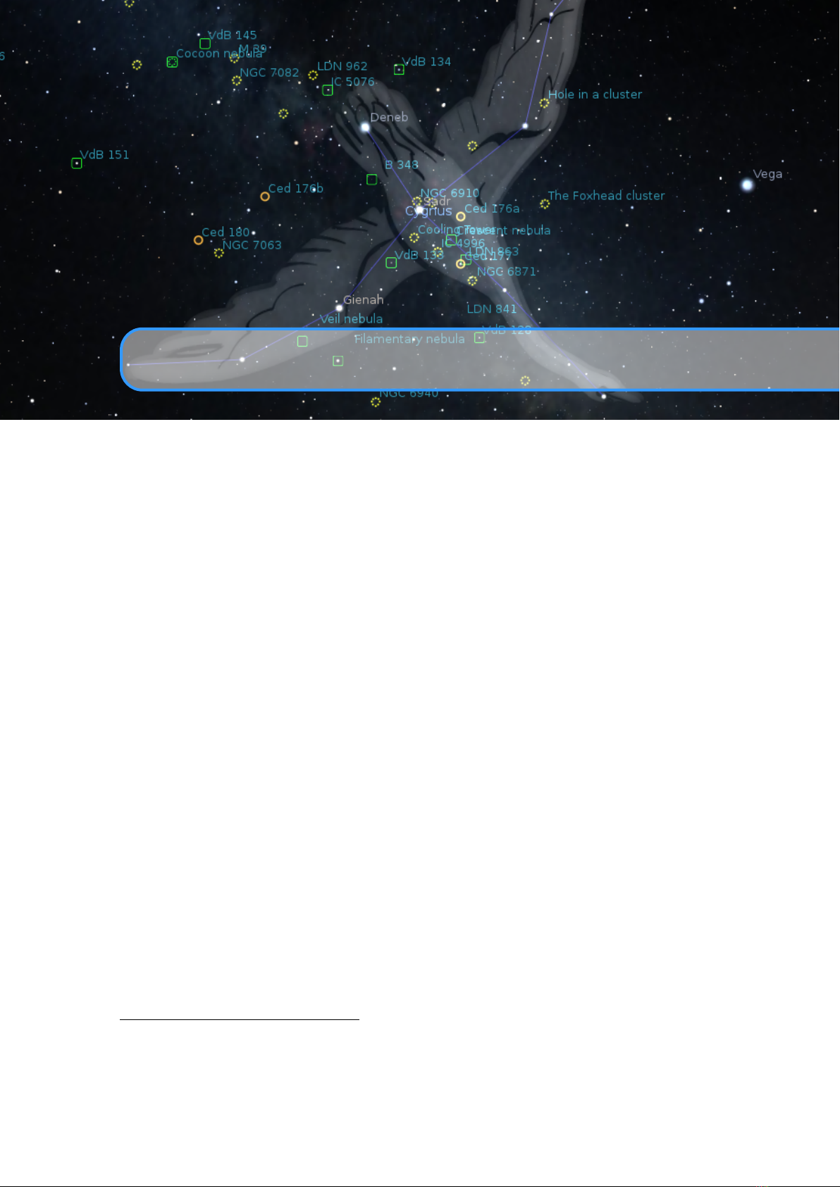
16.4 Mosaic Camera Plugin 247
Figure 16.19: The Mosaic Camera plugin in action. Overlays of LSSTCam(left), DECam (center),
and HyperSuprimeCam (right) are shown, as well as the configuration dialog for the plugin (top
right).
16.4 Mosaic Camera Plugin
JOSH MEYERS
19
16.4.1 Introduction
This plugin overlays an outline of one or more mosaic cameras, i.e., cameras with multiple sensors, onto the
Stellarium celestial sphere. With this functionality, one may compare the fields of view of different cameras,
including potentially one’s own astrophotography setup. Combined with the scripting and remote control
features of Stellarium, various visualizations are possible, including real-time tracking of the observations of
telescopes, playback of past observations, or public outreach demonstrations of the capabilities of various
instruments.
16.4.2 Usage
From the “Cameras” tab of the Mosaic Camera configuration window, you can select from the available
cameras, setting their RA, Dec, rotation, and visibility as desired.
16.4.3 Cameras
Multiple cameras can be individually configured and displayed.
16.4.3.1 Default Cameras
A few cameras come pre-packaged with Stellarium. These are:
19
mailto:jmeyers314@gmail.com

248 Chapter 16. Stellarium at the Telescope
LSSTCam
The largest (as of 2025) digital camera ever assembled at 3.2 gigapixels. Now mounted on the Simonyi
Survey Telescope at the Vera C. Rubin Observatory, this camera will be used to execute the Legacy Survey
of Space and Time, creating a 10-year multicolor ‘movie’ of the southern sky.
Note that the individual CCDs within this camera’s overlay are color-coded by their functionality: Two
shades of blue indicate the main science sensors. (LSSTCam features a hybrid focal plane. Light blue
corresponds to sensors made by Imaging Technology Laboratory, while dark blue corresponds to sensors
made by Imaging Teledyne e2v.) The white sensors in the middle show the field-of-view of the Rubin
Commissioning Camera, a smaller camera used to commission the telescope mount and mirrors before the
main LSSTCam camera was ready. The red sensors in the corners are wavefront sensors, used to monitor
and correct the telescope’s optical alignment in real time. The green sensors are the guider sensors, used to
inform the telescope’s tracking system. See more at
https://rubinobservatory.org/explore/how-r
ubin-works/technology/camera.
HyperSuprimeCam (HSC)
A 900 megapixel camera mounted on the Subaru telescope at the Mauna Kea Observatory. See more at
https://www.naoj.org/Projects/HSC/.
Dark Energy Camera (DECam)
A 570 megapixel camera mounted on the Blanco telescope at the Cerro Tololo Inter-American Observatory.
See more at https://www.darkenergysurvey.org/the-des-project/instrument/.
MegaPrime
A 378 megapixel camera mounted on the Canada-France-Hawaii Telescope at Mauna Kea Observatory. See
more at https://www.cfht.hawaii.edu/Instruments/Imaging/MegaPrime/.
LATISS
The LSST Atmospheric Transmission Imager and Slitless Spectrograph. A 16 megapixel camera mounted
on the Rubin Observatory Auxiliary telescope. See more at
https://rubinobservatory.org/explore
/how-rubin-works/technology/auxtel.
JWST
The James Webb Space Telescope’s focal plane. See more at
https://jwst-docs.stsci.edu/jwst-o
bservatory-hardware/jwst-telescope/jwst-focal-plane#gsc.tab=0.
HST
The Hubble Space Telescope’s focal plane. See more at
https://hst-docs.stsci.edu/acsihb/chapt
er-3-acs-capabilities-design-and-operations/3-1-acs-location-in-the-hst-focal-p
lane.
Roman
The Nancy Grace Roman Space Telescope’s focal plane. See more at
https://roman.gsfc.nasa.gov/
science/WFI_technical.html.
Euclid
The Euclid Space Telescope’s focal plane. See more at
https://www.euclid-ec.org/public/missi
on/vis/.
16.4.3.2 Adding a Camera
When the Mosaic Camera plugin is first enabled, it checks the user data directory for the existence of a
directory
<USERDATA>/modules/MosaicCamera/
. If this directory does not exist, it will be created and
populated with JSON files for each of the default cameras, and one JSON file
camera_order.json
which
specifies the order in which the cameras are displayed.
To add a new camera, create a new JSON file inside this directory, and add a reference to it in the
camera_order.json file.
Camera sensors are specified via their corners, which are assumed to form spherical polygons. The
corners should be specified as gnomonic projections from the sphere to a tangent plane in radians. Multiple
groups of sensors can compose the same camera. For example, LSSTCam has separate sensor groups for
wavefront sensors, guider sensors, and each of two types of science sensors.
Each camera is defined via a JSON file with the structure:
[
{
" ca m e r a _ n ame ": " telesc o p e / camera full name ",
" camera_descr i p t i o n " : " telescope / c amera de s cription in HTML "
} ,

16.4 Mosaic Camera Plugin 249
{
" name ": " name - of - group -1 " ,
" corner s " : [
[
[ corne r 1_x , cor ner 1_y ],
[ corne r 2_x , cor ner 2_y ],
...
] , # senso r 1
[
...
] , # senso r 2
...
]
" color ": {
" value ": [R , G , B , alpha ]
}
} ,
{
" name ": " name - of - group -2 " ,
...
} ,
...
]
See the default camera JSON files for examples.
To reset the plugin to its default state, simply delete the
<USERDATA>/modules/MosaicCamera/
directory.
16.4.4 Control
There are several ways to control the Mosaic Camera plugin.
16.4.4.1 Mosaic Camera Settings Dialog
The Mosaic Camera settings dialog can be opened by right-clicking the MosaicCamera icon, or by selecting
“configure” from the Plugins tab of the main Stellarium Configuration window. This dialog allows you to
configure the cameras, as well as the visibility of the overlays.
16.4.4.2 Keyboard Shortcuts
Keyboard shortcuts (see section 4.8) can be configured to perform the following actions:
•
Cycle the active camera forward or backward
•
Increase or decrease the rotation angle of the current camera by 5 degrees.
•
Set the pointing of the current camera to the current Stellarium view.
•
Toggle the visibility of Mosaic Camera overlays.
•
Toggle the Mosaic Camera settings dialog.
16.4.4.3 Stellarium Scripting
The Mosaic Camera plugin can be controlled via Stellarium’s scripting interface. In the following example,
we set the LSSTCam overlay to be centered at RA=3.0, Dec=4.0 (in J2000 degrees), with a rotation of 1.0
degrees.
MosaicCamera.setCurrentCamera("LSSTCam ")
MosaicCamera.setCurrentRA(3.0)
MosaicCamera.setCurrentDec(4.0)
MosaicCamera.setCurrentRotation(1.0)
an equivalent script is:
MosaicCamera.setRA("LSSTCam ", 3.0)
MosaicCamera.setDec("LSSTCam ", 4.0)
MosaicCamera.setRotation("LSSTCam ", 1.0)
or even:
MosaicCamera.setPosition("LSSTCam ", 3.0, 4.0, 1.0)
16.4.4.4 Stellarium Remote Control
The Mosaic Camera plugin is also accessible via Stellarium’s remote control interface (see 13.7). Here’s a
short python script equivalent to the above example:

250 Chapter 16. Stellarium at the Telescope
import requests
port = 8090 # Default Stellarium port
url = f"http :// localhost :{port }/api/ stelproperty/set"
for name, val in [
["MosaicCamera.currentCamera " , "LSSTCam "],
["MosaicCamera.ra", 3.0],
["MosaicCamera.dec", 4.0],
["MosaicCamera.rotation", 1.0]
]:
requests.post(url, data={"id": name, "value": val})
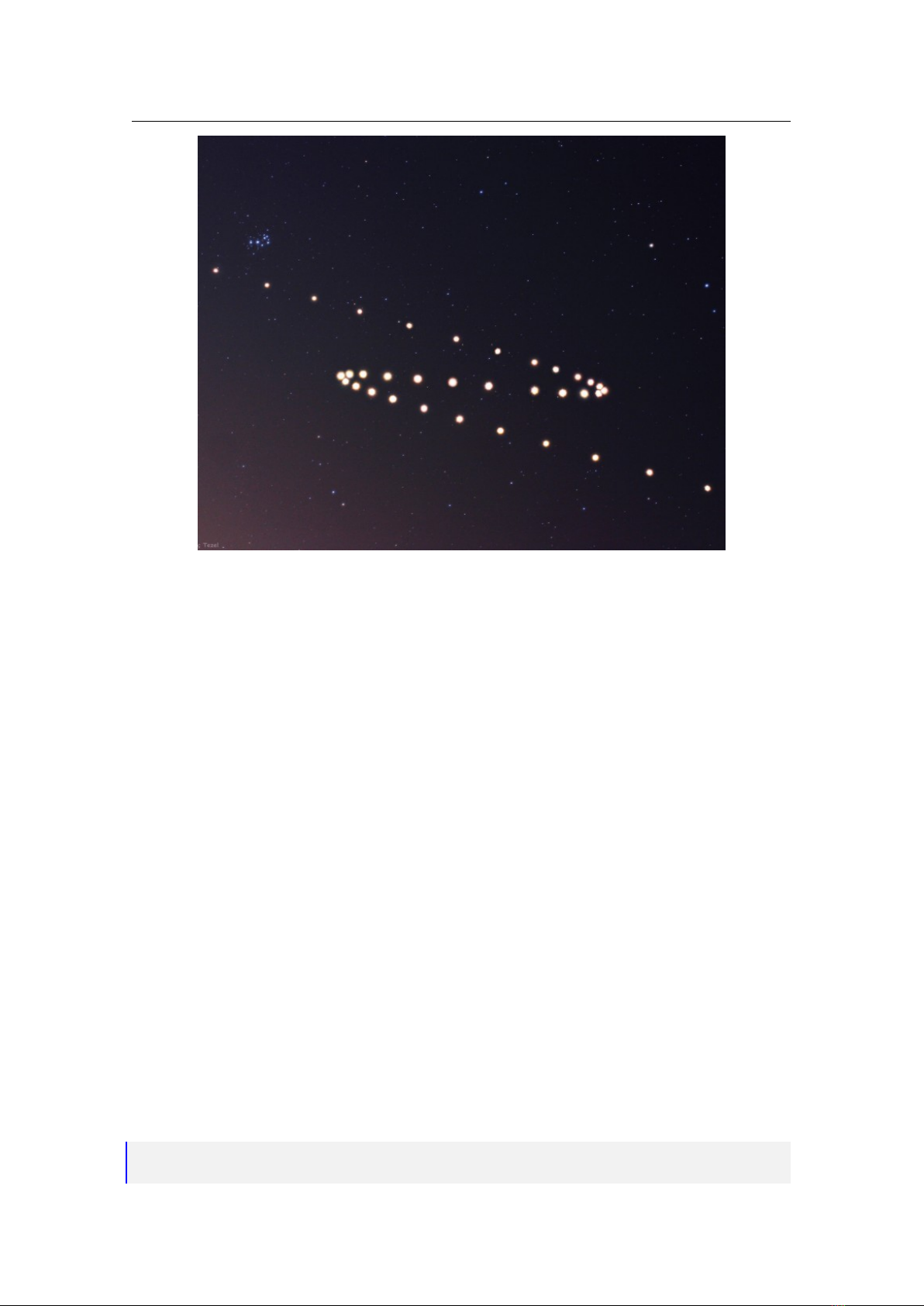
17. Scripting
A. WOLF, G. ZOTTI, WITH ADDITIONS BY WOLFGANG LAUN
17.1 Introduction
The scripting facility is Stellarium’s version of a Presentation, a feature that may be used to run an
astronomical or other show for instruction or entertainment from within the Stellarium program. The use of
scripts was recognized as a perfect way of arranging a presentation of a sequence of astronomical events
from the earliest versions of Stellarium.
The original Stratoscript was quite limited in what it could do, and so a new Stellarium Scripting System
has been developed.
Since version 0.10.1, Stellarium has included a scripting feature based on the Qt5 Scripting Engine
1
.
This made it possible to write small programs within Stellarium to produce automatic presentations, set up
custom configurations, and to automate repetitive tasks. By version 0.14.0 the new scripting engine had
reached a level where it had all required features for usage, and support of scripts for the old Stratoscript
engine has been discontinued.
The programming language ECMAScript
2
(also known as JavaScript) gives users access to all basic
ECMAScript language features such as flow control, variables, string manipulation and so on. Its integration
with Qt’s QtScript module and the way Stellarium’s main components (“StelModule”s) have been designed
to work means that all module functions which are labeled as “slots” can be called from JavaScript.
Interaction with Stellarium-specific features is done via a collection of objects which represent compo-
nents of Stellarium itself. The various modules of Stellarium, and also activated plugins, can be called in
scripts to calculate, move the scene, switch on and off display of objects, etc. You can write text output into
text files with the output() command. You can call all public slots which are documented in the scripting
API documentation
3
.
With the adaptation to Qt6 in versions 1.0 and later we had to switch to yet another scripting engine in
2022. Qt6 comes with QJSEngine
4
, another JavaScript engine which behaves mostly similar to the older
QtScript. However, small differences exist, so that care must be taken if scripts should be developed for
both series of Stellarium. Some older scripts will not work on versions 1.0 and later or at least require some
adaptations described in section 17.5.
1
https://doc.qt.io/qt-5/qtscript-index.html
2
https://en.wikipedia.org/wiki/ECMAScript
3
https://www.stellarium.org/doc/26.0/scripting.html
4
https://doc.qt.io/qt-6/qtjavascript.html

252 Chapter 17. Scripting
17.2 The Script Console
It is possible to load, edit, run and save scripts using the script console window. To toggle the script console,
press
F12
.
17.2.1 The Tabs in the Console
The three tabs “Script”, “Log” and “Output” each provide a text field. In the “Script” text field you can edit a
script, which can be loaded from and saved to a file, and executed. The “Log” text field receives all errors
and other messages resulting from the script’s execution; the “Output” text field will show the results of
core.output() function calls.
The fourth tab, “Settings”, provides some configuration options.
17.2.2 The Menu Bar
The menu bar contains buttons for loading and saving a script. A file dialog is shown for selecting the file.
The “clear” button lets you clear the contents of the text field in the currently selected tab. The drop-down
menu “Execute:” offers a selection of menu entries, mainly intended to let you restore the sky to a clean
state. The entry “selected text as script” executes selected text in the “Script” text field, allowing to test
scripts during development. Entries “remove screen text”, “remove screen images” and “remove screen
markers” remove labels, images and markers, respectively, that may have been left over on the screen from
previous script actions. Each of the “clear map” entries results in a call to
core.clear()
, using one of the
arguments “natural”, “starchart”, “deepspace”, “galactic” or “supergalactic”. These calls reset Stellarium’s
state, resulting in a basic state of the display and providing a clean starting point for another run of your
script.
The button SSC runs the Stellarium Script Preprocessor with the script in the text field as input and
produces an output by recursively inserting all included scripts into the text. This output replaces the contents
of the Script text field. Store the original script if you need it!
17.2.3 German Keyboards
There is a glitch in the keyboard module of the underlying system that is responsible for keyboard handling.
It affects users of Windows and Linux systems with a German, and probably also other international
keyboards: The key combinations
AltGr
+
8
and
AltGr
+
9
cannot be used for typing
[
and
]
. You need
to work around by copy-pasting these two characters. You can also try to use a command line argument like
-platform windows:altgr.
17.3 Includes
Stellarium provides a mechanism for splitting scripts into different files. Typical functions or lists of variables
or celestial objects can be stored in separate
.inc
files and used within other scripts through the include()
command:
include("common_objects .inc");
17.4 Minimal Scripts
This script prints “Hello Universe” in the Script Console log window and into log.txt:
core.debug("Hello Universe");
This script prints “Hello Universe” in the Script Console output window and into the file
output.txt
which
you will also find in the user data directory. The absolute path to the file will also be given in log.txt.
core.output("Hello Universe");
The file
output.txt
will be rewritten on each run of Stellarium. In case you need to save a copy of the
current output file to another file, call
core.saveOutputAs("myImportantData .txt ");
core.resetOutput();
This script uses the LabelMgr module to display “Hello Universe” in red, fontsize 20, on the screen for 3
seconds.

17.5 Critical Scripting Differences introduced with version 1.0 253
var label=LabelMgr.labelScreen("Hello Universe", 200, 200,
true, 20, "#ff0000");
core.wait(3);
LabelMgr.deleteLabel(label);
17.5 Critical Scripting Differences introduced with version 1.0
Qt5’s QtScript module which has been used in versions 0.10 to 0.22 was more flexible and easier to fine-tune
than Qt6’s QJSEngine, which is used in the Qt6-based 1.* series of the program, i.e., versions 1.0 (22.3) and
later. Still, most scripts that have been developed for Stellarium versions 0.10 to 0.22 still run without or
with just minor modifications as described in this section.
17.5.1 Pause/Resume
The Qt6-based builds (version 1.0 and later) do not offer a way to pause and resume a script as was available
in the Qt5-based builds (0.10 to 0.22).
However,
core.waitForKeypress()
can be used to pause a script until a key is pressed, which is
v 26.2
particularly useful for planetarium presentations with a Bluetooth or wireless remote clicker. A visual
indicator “Press key to continue...” can be displayed on screen while the script is paused. To advance, press
SPACE
or the advance key on the remote clicker (which triggers
PgDn
). While the script is paused, you can
operate all other hotkeys (except what you have configured as
SPACE
action).
Example usage:
core.goToObject("Orion");
core.waitForKeypress();
core.goToObject("Sirius");
core.waitForKeypress();
Displaying the “Press key to continue...” message is fine for private use, but may not be wanted in a
show environment. You can switch it off in the Script Console (F12) or in config.ini:
[ scripts ]
fl ag _show_c on tinue_mes sa ge = false
17.5.2 The Vec3f problem
One of the most important little helper classes in the main program are three-dimensional vectors.
Vec3f
describe those with single-precision floating point data, and
Vec3d
are those with double-precision floating
point data.
As late as in version 0.19 we added
Vec3f
and later
Vec3d
data types to the Javascript environment.
These allowed addressing variables of C++ classes
Vec3f
or
Vec3d
with named sub-fields
r
,
g
,
b
(if used to
describe colors), or
x
,
y
,
z
(same data but contextually understood as 3D data). These functions may have
pleased the JavaScript connoisseur when running scripts with Qt5-based builds of Stellarium (series 0.*, and
now usually found on 32-bit and older systems), but we recommend to abstain from their use in new scripts.
Qt6’s scripting module cannot be extended that easily. The
Vec3d
and
Vec3f
data types are not directly
scriptable, but we can deal with method arguments of these types when they are mentioned in the API
documentation (see 17.1). To access internals of these classes, we must use wrapper classes which bear
different names:
V3d can be used where Vec3d must be accessed.
V3f can be used where Vec3f must be accessed.
Color can be used where a Vec3f must be accessed which represents a color value.
They behave slightly different when run using Qt5 or Qt6, as shown in Table 17.1. If you aim for
maximum compatibility between versions, only use the calls which provide equal results in both series. This
current state is far from optimal or even pretty, but a pragmatic solution that works. We invite advanced
developers to find a better solution that works with both Qt5 and Qt6.
17.6 Example: Retrograde motion of Mars
A good way begin writing of scripts: set yourself a specific goal and try to achieve it with the help of few
simple steps. Any complex script can be split into simple parts or tasks, which may solve any newbie

254 Chapter 17. Scripting
Input Result with Qt5 Result with Qt6
x var f1=new V3d(.1,.2,.3);
core.output(f1); [0.1, 0.2, 0.3] V3d(0x249a1cf37c0) [some address]
core.output(+f1.toString()); [0.1, 0.2, 0.3] V3d(0x249a1cf37c0) [some address]
x core.output(f1.toHex()); #19334c #19334c
x core.output(f1.toVec3d()); [0.1, 0.2, 0.3] [0.1, 0.2, 0.3]
x var f2=new V3d(f1.x(), 2*f1.y(), 3*f1.z());
core.output(f2); [0.1, 0.4, 0.9] V3d(0x249a1cf3a60) [some address]
x core.output(f2.toVec3d()); [0.1, 0.4, 0.8999999999999999] [0.1, 0.4, 0.9]
x var crimson=new Color("Crimson");
x core.output(crimson.toHex()); #dc143c #dc143c
core.output(crimson.toVec3f()); [r:0.8627451062202454, g:0.0784313753247261, b:0.23529411852359772] [0.862745, 0.0784314, 0.235294]
core.output(crimson.r); 0.8627451062202454 error
core.output(crimson.r()); error 0.8627451062202454
x core.output(crimson.getR()); 0.8627451062202454 0.8627451062202454
x core.output(crimson.getG()); 0.0784313753247261 0.0784313753247261
x core.output(crimson.getB()); 0.23529411852359772 0.23529411852359772
crimson.g=0.444; (works) (error)
crimson.setG(0.444); (error) (works)
x crimson=new Color(crimson.getR(), 0.444, crimson.getB()); (reassign crimson; recommended for Qt5 and Qt6)
x core.output(crimson.toRGBString()); [r:0.862745, g:0.444, b:0.235294] [r:0.862745, g:0.444, b:0.235294]
x var eq=new Color(GridLinesMgr.getColorEquatorJ2000Grid());
x core.output(eq.toHex()); #00aaff #00aaff
core.output(eq.toVec3f()); [r:0, g:0.6666669845581055, b:1] [0, 0.666667, 1]
core.output(eq.toVec3d()); (n.a.) [0, 0.666667, 1]
core.output(eq.toString()); [0, 0.666667, 1] Color(0x24a11712910) [some address]
x core.output(eq.toRGBString()); [r:0, g:0.666667, b:1] [r:0, g:0.666667, b:1]
x var c=new Color(core.vec3f(.3, .4, .5));
core.output(c.toString()); [0.3, 0.4, 0.5] Color(0x249a1e078b0) [some address]
core.output(c.toVec3f()); [r:0.30000001192092896, g:0.4000000059604645, b:0.5] [0.3, 0.4, 0.5]
x var d=c; // assign to other
core.output(d.toVec3f()); [r:0.30000001192092896, g:0.4000000059604645, b:0.5] [0.3, 0.4, 0.5]
x var c2=new Color(.3, .4, .5);
core.output(c2.toString()); [0.3, 0.4, 0.5] Color(0x24a11712a60) [some address]
core.output(c2.toVec3f()); [r:0.30000001192092896, g:0.4000000059604645, b:0.5] [0.3, 0.4, 0.5]
x var d2=c2; // assign to other
core.output(d2.toVec3f()); [r:0.30000001192092896, g:0.4000000059604645, b:0.5] [0.3, 0.4, 0.5]
Table 17.1: Use of V3d, V3f and Color wrapper classes. Only use the calls marked with x in scripts targeted at all versions of Stellarium.

17.6 Example: Retrograde motion of Mars 255
Figure 17.1: Retrograde motion of Mars in 2005. (Credit & Copyright: Tunc Tezel — APOD: 2006
April 22 – Z is for Mars.)
problems in scripting.
Let me explain it with examples.
Imagine that you have set a goal to make a demonstration of a very beautiful, but longish phenomenon —
the retrograde motion of the planet Mars (Fig. 17.1).
17.6.1 Script header
Any “complex” script should contain a few lines in the first part of the file, which contains important data for
humans — the name of the script and its description — and some rules for Stellarium. You can even assign
default shortcuts in the script header, but make sure you assign a key not used elsewhere! The shortcuts are
read during startup from all scripts in the
scripts
sub-directories of both program and user data directories
(see section 5.2). The description may cover several lines (until the end of the commented header) and should
therefore be the last entry of the header.
//
// Name: Retrograde motion of Mars
// Author: John Doe
// License: Public Domain
// Version: 1.0
// Shortcut : Ctrl+M
// Description : A demo of retrograde motion of Mars.
//
17.6.2 A body of script
At the first stage of writing of the script for a demo of retrograde motion of Mars we should set some limits
for our demo. For example we want to see motion of Mars every day during 250 days since October
1
st
,
2009. Choosing a value of field of view and of the coordinates of the center of the screen should be done at
the this stage also.
Let’s add few lines of code into the script after the header and run it:
core.setDate("2009-10 -01 T10 :00:00");
core.moveToRaDec("08h44m41s ", "+18 d09m13s",1);

256 Chapter 17. Scripting
StelMovementMgr.zoomTo(40, 1);
for (i=0; i<250; i++)
{
core.setDate("+ 1 days ");
core.wait(0.2);
}
Note: The
wait(delay_seconds)
instruction inside the loop is important: when you are just setting the
time in rapid succession, there is no guarantee that the view is updated, or a textual result has been updated
when writing ephemerides, before executing the next time update! The
wait()
ensures the program can
update the main simulation loop and put the planets where they should be at that set time. The minimum
delay required may depend on your computer’s speed.
OK, Stellarium is doing something, but what exactly is it doing? The ground and atmosphere is enabled
and any motion of Mars is invisible. Let’s add an another few lines into the script (hiding the landscape and
atmosphere) after setting date and time:
LandscapeMgr.setFlagLandscape(false);
LandscapeMgr.setFlagAtmosphere(false);
The whole sky is moving now — let’s lock it! Add this line after previous lines:
StelMovementMgr.setFlagLockEquPos(true);
It looks better now, but what about cardinal points, elements of GUI and some “glitch of movement”?
Let’s change the script:
core.setDate("2009-10 -01 T10 :00:00");
LandscapeMgr.setFlagCardinalsPoints(false);
LandscapeMgr.setFlagLandscape(false);
LandscapeMgr.setFlagAtmosphere(false);
core.setGuiVisible(false);
core.moveToRaDec("08h44m41s ", "+18 d09m13s",1);
StelMovementMgr.setFlagLockEquPos(true);
StelMovementMgr.zoomTo(40, 1);
core.wait(2);
for (i=0; i<250; i++)
{
core.setDate("+ 1 days ");
core.wait(0.2);
}
core.setGuiVisible(true);
It’s better, but let’s draw the “path” of Mars! Add those line before the loop:
core.selectObjectByName("Mars", false);
SolarSystem.setFlagIsolatedTrails(true);
SolarSystem.setFlagTrails(true);
Hmm. . . let’s add a few strings with info for users (insert those lines after the header):
var color = "#ff9900";
var info = LabelMgr.labelScreen("A motion of Mars", 20, 20,
false, 24, color);
var apx = LabelMgr.labelScreen("Setup best viewing angle , FOV
and date/ time .", 20, 50, false, 18, color);
LabelMgr.setLabelShow(info, true);
LabelMgr.setLabelShow(apx, true);
core.wait(2);
LabelMgr.setLabelShow(apx, false);
Let’s add some improvements to display info for users — change in the loop:
var label = LabelMgr.labelObject(" Normal motion , West to
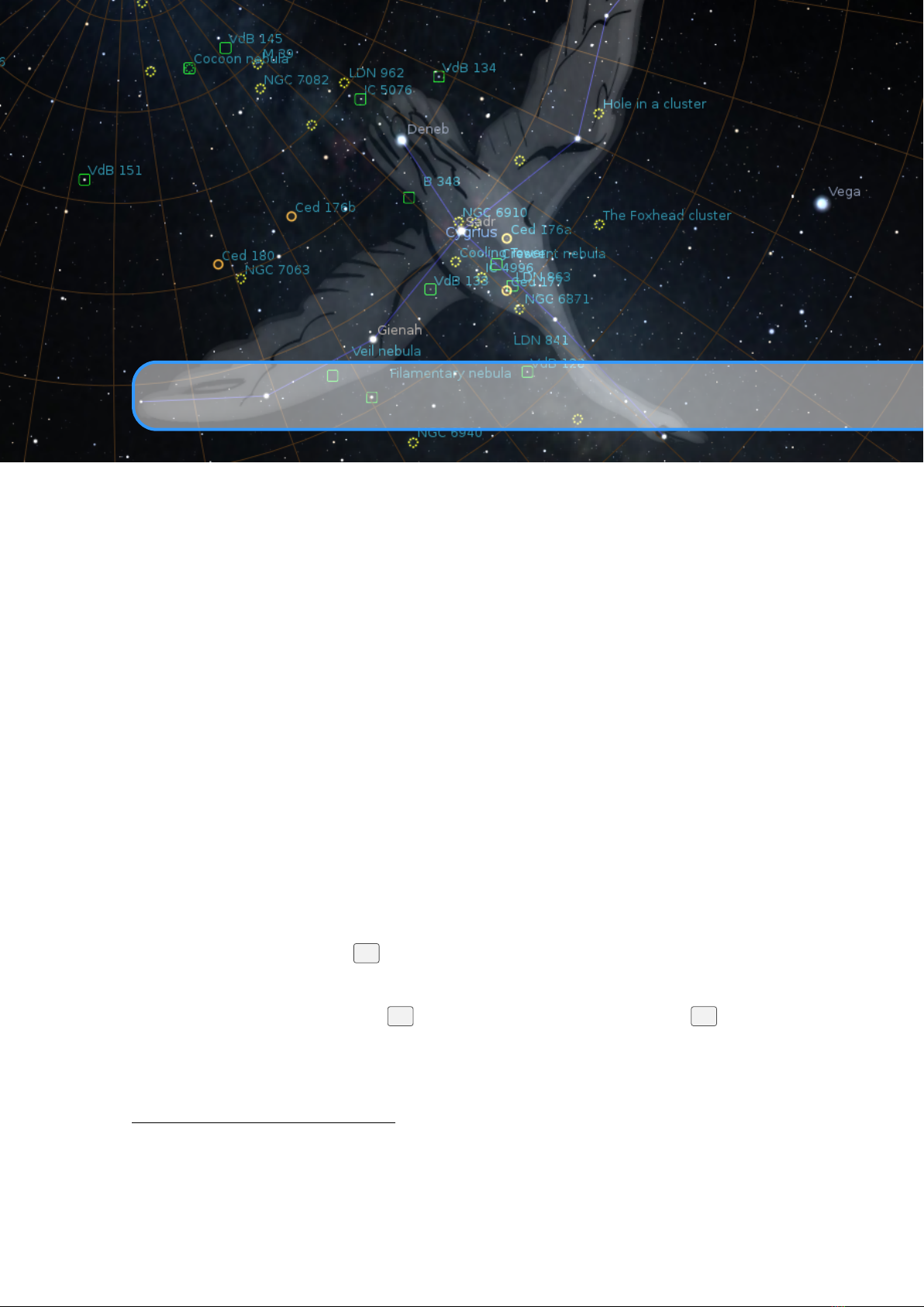
17.7 More Examples 257
East", " Mars ", true, 16, color, "SE");
for (i=0; i<250; i++)
{
core.setDate("+ 1 days ");
if ((i % 10) == 0)
{
var strDate = "Day " + i;
LabelMgr.setLabelShow(apx, false);
var apx = LabelMgr.labelScreen(strDate, 20,
50, false, 16, color);
LabelMgr.setLabelShow(apx, true);
}
if (i == 75)
{
LabelMgr.deleteLabel(label);
label = LabelMgr.labelObject(" Retrograde or
opposite motion begins", " Mars",
true, 16, color, "SE");
core.wait(2);
LabelMgr.deleteLabel(label);
label = LabelMgr.labelObject(" Retrograde
motion " , "Mars ", true, 16, color,
"SE");
}
if (i == 160)
{
LabelMgr.deleteLabel(label);
label = LabelMgr.labelObject(" Normal motion
returns", "Mars ", true, 16, color,
"SE");
core.wait(2);
LabelMgr.deleteLabel(label);
label = LabelMgr.labelObject(" Normal motion",
"Mars ", true, 16, color, "SE");
}
core.wait(0.2);
}
17.7 More Examples
The best source of examples is the
scripts
sub-directory of the main Stellarium source tree. This directory
contains a sub-directory called
tests
which are not installed with Stellarium, but are nonetheless useful
sources of example code for various scripting features.

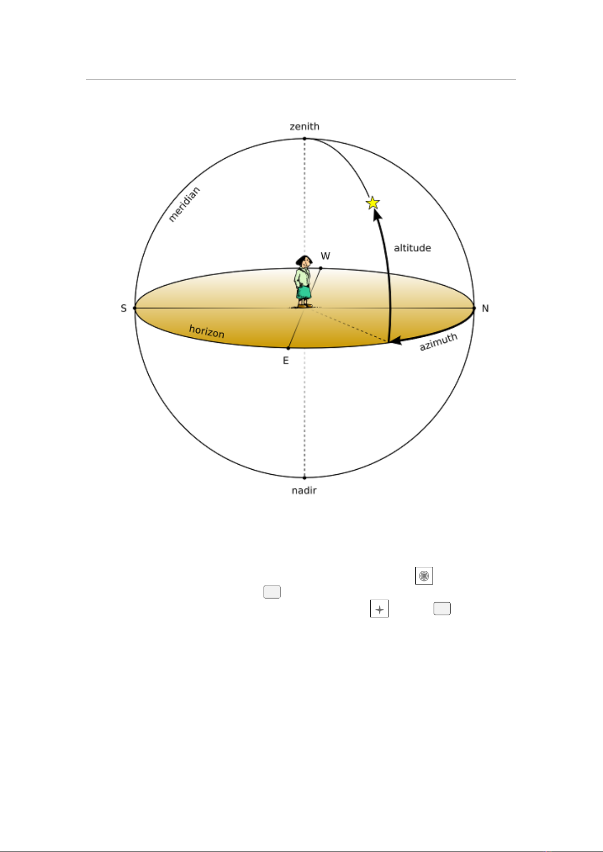
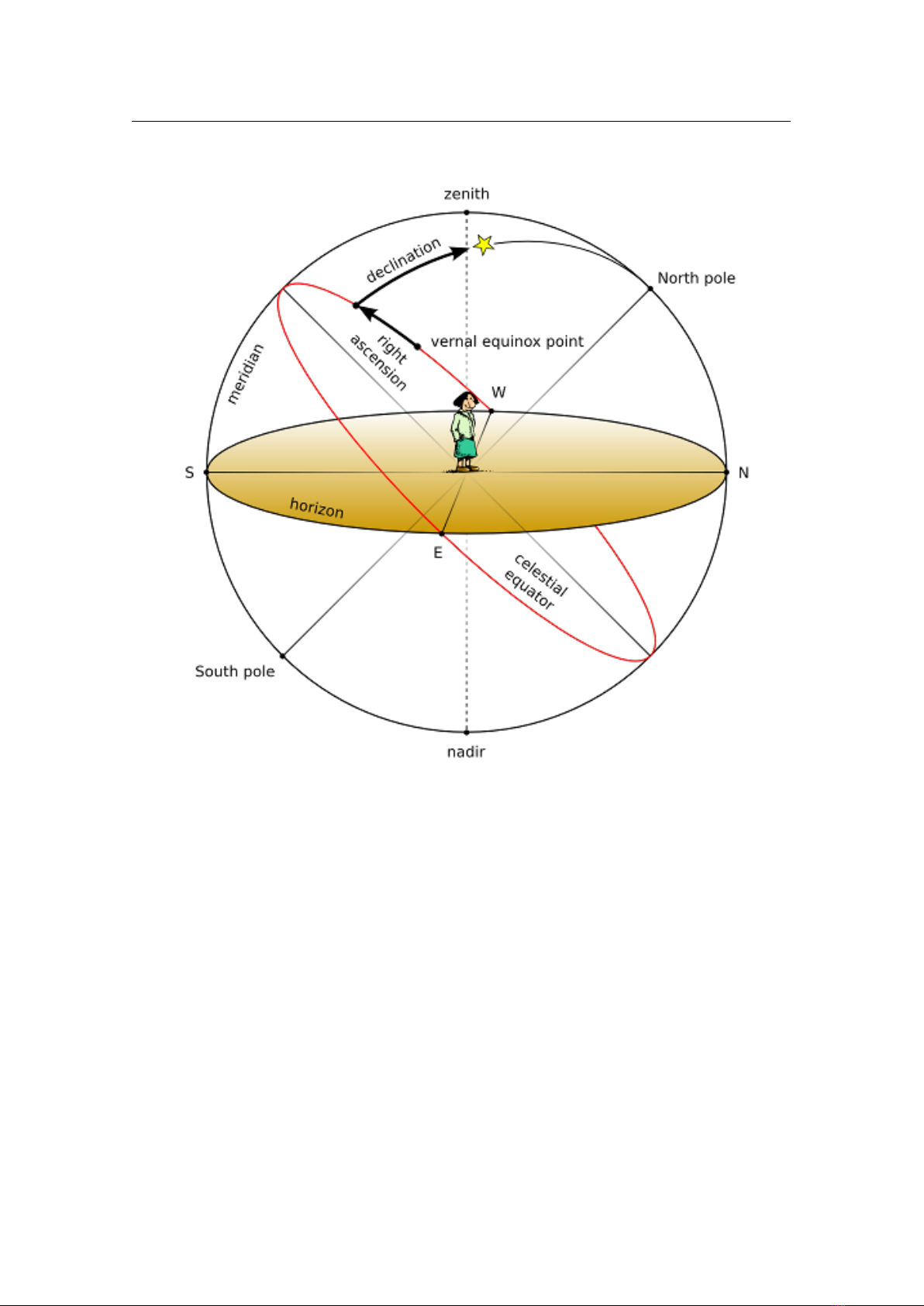

18. Astronomical Concepts
BARRY GERDES, WITH ADDITIONS BY GEORG ZOTTI
This section includes some general notes on astronomy in an effort to outline some concepts that are helpful
to understand features of Stellarium. Material here is only an overview, and the reader is encouraged to get
hold of a couple of good books on the subject. A good place to start is a compact guide and ephemeris such
as the National Audubon Society Field Guide to the Night Sky
1
. Also recommended is a more complete
textbook such as Universe
2
. There are also some nice resources on the net, such as the Wikibooks Astronomy
book
3
.
18.1 The Celestial Sphere
The Celestial Sphere is a concept which helps us think about the positions of objects in the sky. Looking up
at the sky, you might imagine that it is a huge dome or top half of a sphere (a hemisphere), and the stars
are points of light on that sphere. Visualizing the sky in such a manner, it appears that the sphere moves,
taking all the stars with it — it seems to rotate. Watching the movement of the stars we can see that they
seem to rotate around a static point about once a day (the diurnal motion). Stellarium is the perfect tool to
demonstrate this!
1.
Open the location dialog (
F6
). Set the location to be somewhere in mid-northern latitudes. (Just
click on the map to select a location, or fine-tune with the settings.) The United Kingdom is an ideal
location for this demonstration.
2.
Turn off atmospheric rendering
A
and ensure cardinal points are turned on (
Q
). This will keep
the sky dark so the Sun doesn’t prevent us from seeing the motion of the stars when it is above the
horizon.
3. Pan round to point north, and make sure the field of view is about 90°.
4. Pan up so the ‘N’ cardinal point on the horizon is at the bottom of the screen.
5.
Now increase the time rate. Press
K
,
L
,
L
,
L
,
L
– this should set the time rate so the stars
can be seen to rotate around a point in the sky about once every ten seconds. If you watch Stellarium’s
clock you’ll see this is the time it takes for one day to pass at this accelerated rate.
The point which the stars appear to move around is one of the Celestial Poles.
The apparent movement of the stars is due to the rotation of the Earth. Our location as the observer on
the surface of the Earth affects how we perceive the motion of the stars. To an observer standing at Earth’s
North Pole, the stars all seem to rotate around the zenith (the point directly upward). As the observer moves
1
https://www.amazon.com/National-Audubon-Society-Field-Series/dp/0679408525
2
https://www.amazon.com/Universe-Definitive-Visual-Martin-Rees/dp/0756636701
3
https://en.wikibooks.org/wiki/Subject:Astronomy

262 Chapter 18. Astronomical Concepts
south towards the equator, the location of the celestial pole moves down towards the horizon. At the Earth’s
equator, the North Celestial Pole appears to be on the northern horizon.
Similarly, observers in the southern hemisphere see the Southern Celestial Pole at the zenith when they
are at the South Pole, and it moves to the horizon as the observer travels towards the equator.
1.
Leave time moving on nice and fast, and open the configuration window. Go to the location tab and
click on the map right at the top – i.e., set your location to the North Pole. See how the stars rotate
parallel to the horizon, around a point right at the top of the screen. With the field of view set to
90
°
and the horizon at the bottom of the screen, the top of the screen is the zenith.
2. Now click on the map again, this time a little further south. You should see the positions of the stars
jump, and the center of rotation has moved a little further down the screen.
3.
Click on the map even further towards and equator. You should see the centre of rotation having
moved down again.
To help with the visualization of the celestial sphere, turn on the equatorial grid by clicking the button
on the main toolbar or pressing the
E
key. Now you can see grid lines drawn on the sky. These lines are
like lines of longitude and latitude on the Earth, but drawn for the celestial sphere.
The Celestial Equator is the line around the celestial sphere that is half way between the celestial poles –
just as the Earth’s equator is the line half way between the Earth’s poles.
18.2 Coordinate Systems
18.2.1 Altitude/Azimuth Coordinates
The Horizontal Coordinate System (also called Altitude/Azimuth coordinate system) can be used to describe
a direction of view (the azimuth angle) and an angular height in the sky (the altitude angle). The azimuth
angle is measured clockwise round from due north
4
. Hence North itself is 0°, East
90
°, Southwest is
225
°
and so on. The altitude angle is measured up from the mathematical horizon, which is just halfway between
“straight up” and “straight down”, without regard to the landscape. Looking directly up (at the zenith) would
be
90
°, half way between the zenith and the horizon is
45
° and so on. The point opposite the zenith is called
the nadir.
The Altitude/Azimuth coordinate system is attractive in that it is intuitive – most people are familiar
with azimuth angles from bearings in the context of navigation, and the altitude angle is something most
people can visualise pretty easily.
However, the altitude/azimuth coordinate system is not suitable for describing the general position of
stars and other objects in the sky – the altitude and azimuth values for a celestial object change with time and
the location of the observer.
Stellarium can draw grid lines for altitude/azimuth coordinates. Use the button on the main toolbar
to activate this grid, or press the
Z
key.
In addition, the cardinal points can be highlighted using the
button or
Q
key.
There are a few great circles with special names which Stellarium can draw (see section 4.4.4).
Meridian
This is a great circle which runs through the North Pole towards the zenith and further to the
South Pole and nadir.
(Mathematical) Horizon This is the line exactly 90° away from the zenith.
First Vertical
This is the vertical circle perpendicular to the horizon and which runs from the East point
through the zenith, down the West point and to the nadir.
18.2.2 Right Ascension/Declination Coordinates
Like the Altitude/Azimuth system, the Right Ascension/Declination (RA/Dec) Coordinate System (or
Equatorial Coordinate System) uses two angles to describe positions in the sky. These angles are measured
from standard points on the celestial sphere. Right ascension
α
and declination
δ
are to the celestial sphere
what longitude and latitude are to terrestrial map makers.
The Northern Celestial Pole has a declination of
δ = 90
°, the celestial equator has a declination of
δ = 0
°,
and the Southern Celestial Pole has a declination of δ = −90°.
Occasionally, instrument makers of the past may have engraved polar distance
p
instead:
p = 90
○
− δ
.
Stellarium can be configured to use this convention, see section 4.3.3.v 25.4
4
In some textbooks azimuth is counted from south. There is no global authority to decide upon this issue, just be
aware of this when you compare numbers with other sources.

18.2 Coordinate Systems 263
Figure 18.1: Altitude/Azimuth (Horizontal) Coordinate System
Right ascension is measured as an angle round from the vernal equinox, a point in the sky also known as
the First Point of Aries
à
, in the same way that longitude is measured around the Earth from Greenwich.
Figure 18.2 illustrates RA/Dec coordinates. The angle
α
is usually expressed as time with minute and
seconds, with 15° equaling one hour.
Unlike Altitude/Azimuth coordinates, RA/Dec coordinates of a star do not change when the observer
changes latitude, and do not change noticeably over the course of the day due to the rotation of the Earth.
RA/Dec coordinates are generally used nowadays in star catalogs such as the Hipparcos catalog.
However, the story is complicated a little by precession (section 18.8) and parallax (section 18.9).
Precession causes a slow drift of the coordinates almost parallel to the ecliptic, and therefore star catalogs
always have to specify their equinox of validity.
Current catalogs and atlases use coordinates for the standard epoch J2000.0. The currently best defined
coordinate system, the International Celestial Reference Frame (ICRF), is one particular version described in
detail in the astronomical literature (Urban and Seidelmann, 2013). Other catalogs with data referring to
“J2000.0” may have to be slightly adjusted (usually in sub-arcsecond rotations) to match the ICRF coordinate
system (short ICRS).
Stars close to the celestial poles are permanently visible above the horizon and thus called circumpolar.
Those stars have observable upper and lower culminations when they pass the meridian arc spanning from
the celestial pole over the zenith to the opposite point on the horizon, or from the celestial pole to the horizon
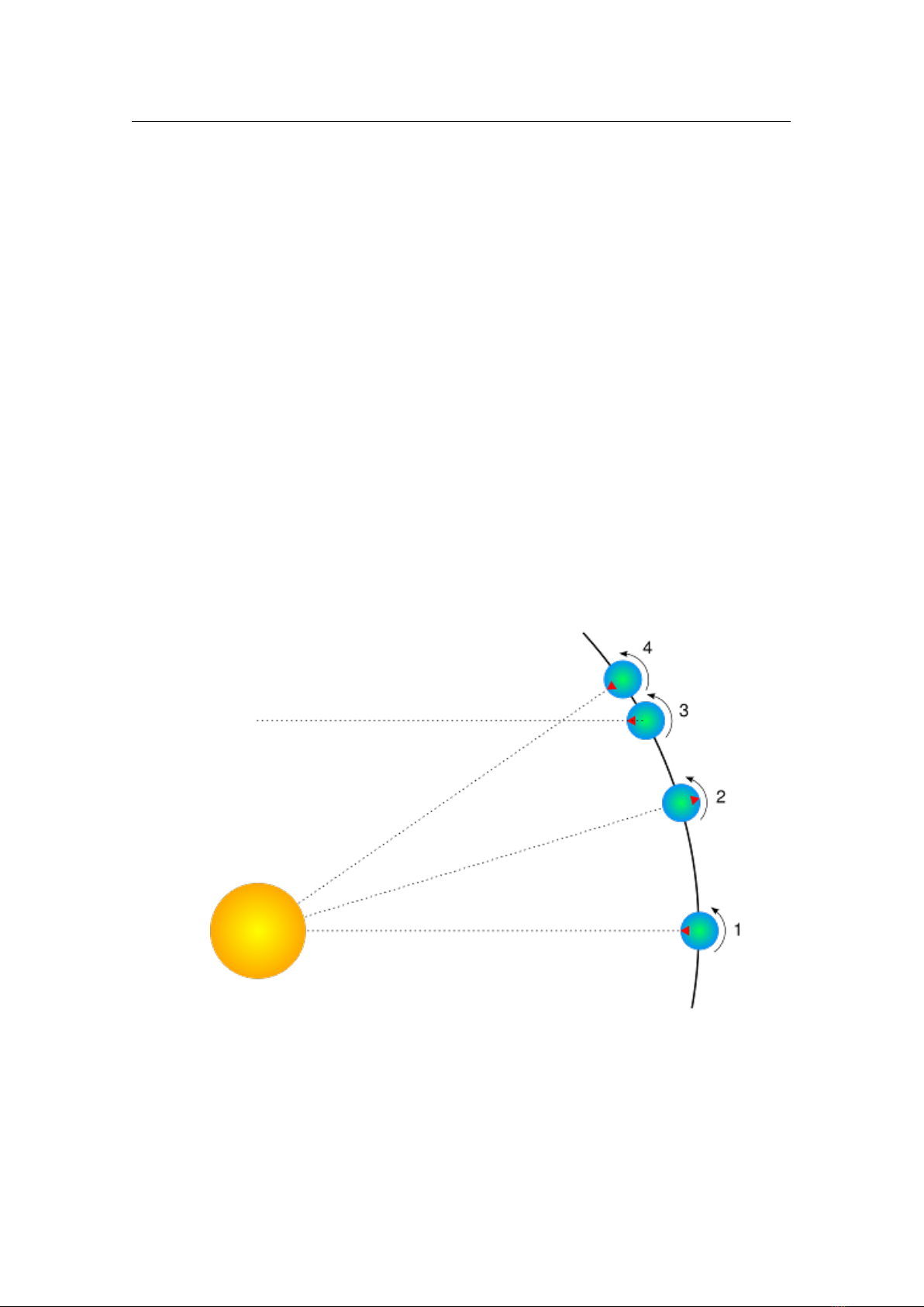
264 Chapter 18. Astronomical Concepts
Figure 18.2: Equatorial Coordinates
below, respectively.
Those circumpolar stars which show their upper culmination between pole and zenith also have limits in
azimuth which they can reach in their daily course, the points of greatest digression. At these points they
move vertically upwards (in the east) or downwards (in the west), respectively.
Stellarium can draw grid lines for equatorial coordinates. Use the button on the main toolbar to
activate this grid, or press the
E
key to draw the equatorial grid for the simulation time. The Markings
dialog (4.4.4) allows you to set also the grid for J2000.0 standard coordinates.
There are again a few great circles with special names which Stellarium can draw in addition, both for
simulation time and for J2000.0 (see section 4.4.4).
Celestial Equator the line directly above the Earth’s (or more generally, the observer’s planet’s) equator.
Colures
These are lines similar to meridian and first vertical in the azimuthal system. The Equinoctial
Colure runs from the North Celestial Pole NCP through the First Point of Aries
à
, South Celestial
Pole SCP and First Point of Libra
æ
, while the Solstitial Colure runs from the NCP through First
Point of Cancer ã, SCP and First Point of Capricorn é.
In case you are observing from another celestial object, the equatorial coordinates use a system similar
to the one referring to the Earth-based coordinates, but parallel to the planet’s rotational axis.

18.2 Coordinate Systems 265
18.2.3 Fixed Equatorial Coordinates
The celestial sphere with its stars and other objects located in equatorial coordinates seems to rotate around
the celestial polar axis. When observing with a telescope, it proved useful to mount the instrument on an axis
which is aimed to be parallel to the earth’s axis, i.e., points to the celestial pole. In this case, after setting
the objects’s declination, it is enough to move the telescope around this polar axis to track its course over
time and keep the object in the field of view. We can describe the Fixed Equatorial Coordinate System as an
intermediate coordinate system which uses the same equator and declination as the equatorial system, but
does not rotate as time goes by. The longitudinal coordinate is conventionally counted in 0. . . 24 hours from
the meridian (0h) along the celestial equator towards the west (6h) and is aptly named Hour Angle. A star
which has passed the meridian will reach hour angle of 1 hour one sidereal hour later. In some traditions,
decimal degrees may be preferred, and negative hour angles are used instead on the eastern half of the sky.
(See section 4.3.3 for settings.)
Stellarium can display the fixed equatorial coordinates in the Markings dialog (4.4.4).
18.2.4 Ecliptical Coordinates
The Earth’s orbit around the Sun, i.e., the ecliptic, defines the “equatorial line” of this coordinate system,
which is traditionally used when computing the coordinates for planets because of their close proximity to
this line. Mirroring Earth’s motion, the Sun is seen to move along the ecliptic.
The zero point of ecliptical longitude
λ
is the same as for equatorial coordinates (
à
), and the ecliptical
latitude β is counted positive towards the Northern Ecliptical Pole NEP in the constellation of Draco.
Moon and Sun (and to a much lesser extent, the other planets) pull on the equatorial bulge and try to
put Earth’s axis normal to its orbital plane. Earth acts like a spinning top and evades this pull in a sideways
motion, so that Earth’s axis seems to describe a small circle over a period of almost 26.000 years (see
section 18.8).
In addition, ecliptic obliquity against the equatorial coordinates, which mirrors the Earth’s axial tilt,
slowly changes.
Therefore, also for ecliptical coordinates it is required to specify which date (epoch) the coordinates
refer to. Stellarium can draw grids for two epochs. Use the
,
key to draw the ecliptic for the simulation
time. The Markings dialog (4.4.4) allows you to add date marks to the ecliptic line and also show a line for
v 23.1
epoch J2000.0 and grids for the ecliptical coordinates for current epoch and epoch J2000.0. You can assign
your own shortcut keys (section 4.8) if you frequently operate with these coordinates.
Since version 0.14.0 Stellarium can very accurately show the motions between the coordinate sys-
tems (Vondrák, Capitaine, and Wallace, 2011; Vondrák, Capitaine, and Wallace, 2012), and it is quite
interesting to follow these motions for several millennia. To support such demonstrations, Stellarium can also
draw the precession circles between celestial and ecliptical poles (activate them in the Markings dialog (4.4.4).
However, these circles are simply plotted centered on the instantaneous ecliptic pole by the instantaneous
value of obliquity. If you observe long enough, you will see that these circles vary in size, reflecting the
changes in ecliptic obliquity. The real track of where Earth’s axis is pointing forms an open helical loop.
The inner planets are best observed when their apparent distance from the Sun, or elongation, reaches a
maximum. Unfortunately there are two definitions for elongation, though:
ψ angular distance on the sphere. This is today the most widely used definition.
∆
λ
À
difference between solar and the object’s ecliptical longitude. The advantage of using this definition
is that we can easily read opposition (
∆λ
À
= 180
○
) and conjunction (
∆λ
À
= 0
○
). We can also see
whether we have eastern elongation (
∆λ
À
> 0
) where the planet is visible in the evening sky, or
western elongation (
∆λ
À
< 0
) where the planet is visible in the morning sky. For the inner planets
Mercury and Venus we further discern superior conjunction, when the planet is “above”, or behind,
the Sun, and inferior conjunction, when the planet is “below”, or closer than, the Sun.
Many of the minor bodies are best observed around the times of their opposition. Stellarium can display
a great circle in the ecliptical coordinates which runs through the ecliptic poles and through the Sun, thereby
allowing to estimate opposition and conjunction. Activate display of this Opposition/Conjunction Line in the
Markings dialog (Labeled “O./C. longitude”; 4.4.4). The Markings dialog also provides the possibility to
visualize the antisolar point, which lies opposite of the Sun, on the intersection of the ecliptic and the O/C
line.
Another interesting aspect of planets is their quadrature from the Sun. Here their angular distance is
90
○
. You can activate display of the quadrature circle in the Markings dialog (4.4.4).
It is interesting to note that star catalogs before TYCHO BRAHE’s (1546–1601), most notably the one in
PTOLEMY’s Almagest, used ecliptical coordinates. The reason is simple: it was known since HIPPARCHUS

266 Chapter 18. Astronomical Concepts
that stellar coordinates slowly move along the ecliptic through precession, and the correction to coordinates
of a date of interest was a simple addition of a linear correction to the ecliptical longitude in the catalog.
Changes of ecliptic obliquity were discovered much later.
18.2.5 Galactic Coordinates
The Milky Way appears to run along a great circle over the sky, mirroring the fact that the Sun is a star in it.
Coordinates for non-stellar objects which belong to the Milky Way like pulsars or planetary nebulae are
often mapped in Galactic Coordinates, where galactic longitude
l
and galactic latitude
b
are usually given
in decimal degrees. Here, the zero point of galactic longitudes lies in the Galactic Center.
Stellarium can also draw a galactic grid and the galactic equator by activating the respective options
in the Markings dialog (see section 4.4.4). You can assign a keyboard shortcut if you frequently use these
coordinates (see 4.8).
18.2.6 Planet Coordinates
The larger objects in the Solar system are described as spheroids, sometimes flattened into slightly ellipsoid
shape.
Just like the Prime Meridian on Earth has been defined to run through Greenwich Observatory, each such
object in the Solar system for which any kind of rotation has been detected has a prime meridian defined by
the IAU Working Group on Cartographic Coordinates and Rotational Elements (WGCCRE). On a rocky
planet this is usually defined by some surface feature like a crater. For the Moon, it has traditionally been
the center of the Lunar disk. For the gas giant planets with ever-changing atmospheric features, there are
even several systems of rotation. Most notably on Jupiter, System I describes the rotation of its equatorial
area, while System II describes the mean atmospheric rotation north of the south component of the north
equatorial belt, and south of the north component of the south equatorial belt. Official sources prefer to list
the rotation of the magnetic fields (System III) for these planets. The most interesting feature on Jupiter for
most observers is the Great Red Spot (GRS), a huge storm that has been observed since the 19th, if not even
since the 17th century.
Astronomical almanacs and observing guides often list transit times when the GRS crosses the center of
Jupiter’s visible disk. Stellarium aims to show it at the right place. The storm moves in longitude, and to
adjust for this you can configure its System II longitude in the settings, see 4.4.2.
Like many planet moons, also Earth’s Moon shows one side towards its planet. However, given its
elliptical orbit and disturbations by Earth, Sun and other planets, the Moon seems to nod slightly in east-west
and north-south directions. This motion is called Libration. Stellarium gives geocentric libration in longitude
L
and latitude
B
, which are the coordinates of the apparent center of the Lunar disk. Another way to express
this shift is the total angle of libration and the direction into which the Moon’s mean center has been shifted.
This angle is given counterclockwise from the direction of the North pole on the Lunar disk. The larger this
shift is, the better you can observe the opposite side, which is therefore marked in brackets. If libration is
larger than 3/5/7 degrees, Stellarium shows 1, 2 or 3 exclamation marks to draw your attention further to this
lunar rim. However, you also need light on this edge.
Another interesting point for which Stellarium gives coordinates is the sub-solar point (L
s
, B
s
).
The Selenographic colongitude of the Sun
c
0
= 450
○
− L
s
is given for the Moon. This helps estimating
the terminator (Meeus, 1998):
•
The morning terminator is at 360
○
− c
0
.
•
The evening terminator is at 180
○
− c
0
.
•
When c
0
= 0
○
, the Sun rises at selenographic longitude L = 0
○
, near First Quarter.
•
When c
0
= 90
○
, the Sun rises at selenographic longitude L = 270
○
, near Full Moon.
•
When c
0
= 180
○
, the Sun rises at selenographic longitude L = 180
○
, near Last Quarter.
•
When c
0
= 270
○
, the Sun rises at selenographic longitude L = 90
○
, near New Moon.
c
0
is used to compute the Sun’s altitude
h
over a surface point, e.g. a crater on the Moon at position
(η, θ ), which is displayed when you select a surface feature.
sinh = sinB
s
sin
θ + cosB
s
cosθ sin(c
0
+ η) (18.1)
18.3 Distance
As DOUGLAS ADAMS (1952–2001) pointed out in The Hitchhiker’s Guide to the Galaxy (Adams, 1981),

18.4 Time 267
Space [. . . ] is big. Really big. You just won’t believe how vastly, hugely, mind-bogglingly
big it is. I mean, you may think it’s a long way down the road to the chemist, but that’s just
peanuts to space.[p.76]
Astronomers use a variety of units for distance that make sense in the context of the mind-boggling vastness
of space.
Astronomical Unit (AU)
This is the mean Earth-Sun distance. Roughly 150 million kilometers (
1.49598×
10
8
km
). The AU is used mainly when discussing the solar system – for example the distance of
various planets from the Sun.
Light year (LY) A light year is not, as some people believe, a measure of time. It is the distance that light
travels in a year. The speed of light being approximately 300,000 kilometers per second means a light
year is a very large distance indeed, working out at about 9.5 trillion kilometers (
9.46073× 10
12
km
).
Light years are most frequently used when describing the distance of stars and galaxies or the sizes of
large-scale objects like galaxies, nebulae etc.
Parsec (pc)
A parsec is defined as the distance of an object that has an annual parallax of 1 second of
arc. This equates to 3.26156 light years (
3.08568× 10
13
km
). Parsecs (and derivatives: kiloparsec
kpc
, megaparsec
Mpc
) are most frequently used when describing the distance of stars or the sizes of
large-scale objects like galaxies, nebulae etc.
18.4 Time
Figure 18.3: Sidereal day
The length of a day is defined as the amount of time that it takes for the Sun to travel from the highest
point in the sky at mid-day to the next high-point on the next day. In astronomy this is called a solar day.
The apparent motion of the Sun is caused by the rotation of the Earth. However, in this time, the Earth not
only spins, it also moves slightly round its orbit. Thus in one solar day the Earth does not spin exactly
360
°
on its axis. Another way to measure day length is to consider how long it takes for the Earth to rotate exactly
360°. This is known as one sidereal day.
Figure 18.3 illustrates the motion of the Earth as seen looking down on the Earth orbiting the Sun. The
red triangle on the Earth represents the location of an observer. The figure shows the Earth at four times:
1. The Sun is directly overhead - it is mid-day.

268 Chapter 18. Astronomical Concepts
2.
Twelve hours have passed since 1. The Earth has rotated round and the observer is on the opposite
side of the Earth from the Sun. It is mid-night. The Earth has also moved round in its orbit a little.
3. The Earth has rotated exactly 360°. Exactly one sidereal day has passed since 1.
4.
It is mid-day again – exactly one solar day since 1. Note that the Earth has rotated more than
360
°
since 1.
It should be noted that in figure 18.3 the sizes of the Sun and Earth and not to scale. More importantly, the
distance the Earth moves around its orbit is much exaggerated. The Earth takes a year to travel round the
Sun – 365
1
4
solar days. The length of a sidereal day is about 23 hours, 56 minutes and 4 seconds.
18.4.1 Sidereal Time
It takes exactly one sidereal day for the celestial sphere to make one revolution in the sky. Astronomers find
sidereal time useful when observing. This is the Right Ascension which is currently passing the meridian
line, or, equivalent, the Hour Angle of the First Point of Aries à. When visiting observatories, look out for
doctored alarm clocks that have been set to run faster and show sidereal time!
18.4.2 Julian Day Number
In the 19th century, astronomer JOHN HERSCHEL (1792–1871) introduced the use of Julian Day numbers
(invented around the time of the Gregorian calendar reform). This is a simple continuous day count starting
on January 1, -4712 (4713 BC). There are no years, months etc., and the integral day number switches at
noon, so during a single night of observation (in Europe) the date never changes.
The fractional part of the number is just the fraction of day that has elapsed since last noon. Given that a
day has 86400 seconds, we should give a JD with 5 decimal places to capture the nearest second.
This causes a problem for modern computers: even a “double precision float” can keep only about
13 decimal places. More than 2.4 million days have passed, so that e.g. January 1, 2000, 12:00UT is
2451545.0, which is an accurately storable number with 7 decimal places, but 12:34:56UT is computed
as 2451545.02426. A more accurate result would yield 2451545.024259259259... So, for a field where
sub-second accuracy became crucial like spacecraft operations, the Modified Julian Day (MJD) has been
introduced. It is simply
MJD = JD − 2400000.5. (18.2)
This means, days start at midnight, and the (constant, in our era) decimal places of the “big numbers” at the
begin of the number have been traded in for more decimal places at the end.
Don’t put your expectations too high when you see MJD displayed (section 4.1): Stellarium uses a
double-precision floating point number for JD for internal timekeeping, and Stellarium’s display of MJD is
simply computed from it. So you cannot set temporal increments smaller than a second, and it hardly would
make sense to expect more accuracy from the simulation algorithms.
18.4.3 Delta T
Until around 1900, the Earth’s rotation was regarded as perfect standard of time. There were 86400 seconds
per mean solar day, and the accuracy of reproducing time with mechanical clocks only in this time started to
become as good as the Earth’s rotation itself.
Astronomers who computed solar eclipses reported in texts from antiquity wondered about a required
time shift which they originally attributed to a yet-unknown “secular acceleration of the lunar motion”.
However, it turned out that indeed the gravitational effect of the Moon which causes the tides also has effects
on Earth’s rotation: the tides slowly break Earth’s rotational speed. The energy is also transferred to the
Moon, and the acceleration leads to the Moon slowly moving away from the Earth
5
.
This led to the introduction of a time named Ephemeris Time (ET) with progresses in the speed of the
second in the year 1900, to be used for positional computation in our solar system, in addition to Greenwich
Mean Time (GMT), from which all zone times and “civil” clock times were derived.
The introduction of atomic clocks in the middle of the 20th century led to a redefinition of the (temporal)
second, which has been de-coupled from Earth’s rotation. This time, the International Atomic Time TAI
6
, is
5
No need to worry, the Moon recedes from the Earth only a few centimeters per year as measured with the laser
reflectors left by the Apollo astronauts in the 1970s. In a very far future, however, there will only be annular solar
eclipses as a consequence!
6
From the French name temps atomique international

18.4 Time 269
the basis for Terrestrial Time TT which can be considered as constantly progressing at constant speed
7
, and
is used for computation of the planetary positions.
Still, people living on Earth prefer to have the mean solar noon governing the run of day and night.
Therefore all forms of civil time are linked to Coordinated Universal Time UTC. Seconds in UTC and
TAI are of equal length. The slow and irregular divergence between TAI and UTC is observed by a few
standardization institutes. When necessary, a leap second can be introduced to the UTC to bring the Earth’s
rotation back in sync so that the Mean Sun again culminates at noon.
The difference
∆T = T T − UT
(or “Delta T”) describes the temporal offset which amounts already to
more than a minute in the 21st century. There have been many attempts to properly model
∆T
, and Stellarium
offers several models you can choose from in the configuration dialog (see section 4.3.4). “Espenak and
Meeus (2006, 2014)”, is a widely accepted standard. The default, “Modified Espenak and Meeus (2006,
2014, 2023)”, is created to make
∆T
closely in line with observed and predicted values between the years
2015-2050. But if you are a researcher and want to experiment with alternative models, you will hopefully
like this feature. you can even specify your own data for
a
,
b
,
c
,
y
and the secular term for lunar acceleration
n (actually ˙n = dndt in units of arcsecondscentury
2
) if you can model ∆T according to the formula
∆T = a + b ⋅ u + c⋅ u
2
where (18.3)
u =
year− y
100
(18.4)
18.4.3.1 List of ∆T models in Stellar ium
The following list describes sources and a few details about the models for ∆T implemented in Stellarium.
Without correction. Correction is disabled. Use only if you know what you are doing!
Schoch (1931).
This historical formula was obtained by Schoch (1931) and was also used in “A New Test of
Einstein’s Theory of Relativity by Ancient Solar Eclipses” (Henriksson, 2009). See for more in Peters
(2010). ˙n = −29.68
′′
cy
2
.
Clemence (1948).
This empirical equation was published in “On the system of astronomical constants”
(Clemence, 1948). Valid range of usage: between years 1681 and 1900. ˙n = −22.44
′′
cy
2
.
IAU (1952).
This formula is based on a study of post-1650 observations of the Sun, the Moon and the
planets (Spencer Jones, 1939) and reproduced in Astronomical Formulae for Calculators (Meeus,
1988). It was also adopted in the PC program SunTracker Pro. Valid range of usage: between years
1681 and 1936. ˙n = −22.44
′′
cy
2
.
Astronomical Ephemeris (1960).
This is a slightly modified version of the IAU 1952 (Spencer Jones,
1939) formula which was adopted in the “Astronomical Ephemeris” (Wilkins, 1961) and in the Canon
of Solar Eclipses -2003 to +2526 (Mucke and Meeus, 1983). Valid range of usage: between years
-500 and 2000. ˙n = −22.44
′′
cy
2
.
Tuckerman (1962, 1964) & Goldstine (1973).
The famous tables (Tuckerman, 1962; Tuckerman, 1964)
list the positions of the Sun, the Moon and the planets at 5- and 10-day intervals from 601 BCE to
1649 CE. The same relation was also implicitly adopted in the syzygy tables of Goldstine (1973).
Valid range of usage: between years -600 and 1649.
Muller & Stephenson (1975).
This equation was published in “The accelerations of the earth and moon
from early astronomical observations” (Muller and F. R. Stephenson, 1975). Valid range of usage:
between years -1375 and 1975. ˙n = −37.5
′′
cy
2
.
Stephenson (1978).
This equation was published in “Pre-Telescopic Astronomical Observations” (F. R.
Stephenson, 1978). ˙n = −30.0
′′
cy
2
.
Schmadel & Zech (1979).
This 12th-order polynomial equation (outdated and superseded by Schmadel
and Zech (1988)) was published in “Polynomial approximations for the correction delta T E.T.-U.T. in
the period 1800-1975” (Schmadel and Zech, 1979) as fit through data published by Brouwer (1952).
Valid range of usage: between years 1800 and 1975, with meaningless values outside this range.
˙n = −23.8946
′′
cy
2
.
Morrison & Stephenson (1982).
This algorithm Morrison and F. R. Stephenson, 1982 was adopted in
Planetary Programs and Tables from –4000 to +2800 (Pierre Bretagnon and Simon, 1986) and
in the PC planetarium program RedShift. Valid range of usage: between years -4000 and 2800.
˙n = −26.0
′′
cy
2
.
7
We don’t discuss relativity here. The advanced reader is referred to the presentation in the Wikipedia,
https:
//en.wikipedia.org/wiki/Delta_T.

270 Chapter 18. Astronomical Concepts
Stephenson & Morrison (1984).
This formula was published in “Long-term changes in the rotation of the
earth - 700 B.C. to A.D. 1980” (F. R. Stephenson and Morrison, 1984). Valid range of usage: between
years -391 and 1600. ˙n = −26.0
′′
cy
2
.
Stephenson & Houlden (1986).
This algorithm (Houlden and F. Stephenson, 1986) is used in the PC
planetarium program Guide 7. Valid range of usage: between years -600 and 1600.
˙n = −26.0
′′
cy
2
.
Espenak (1987, 1989).
This algorithm was given in Fifty Year Canon of Solar Eclipses: 1986 – 2035
(Espenak, 1987) and in Fifty Year Canon of Lunar Eclipses: 1986 – 2035 (Espenak, 1989). Valid
range of usage: between years 1950 and 2100.
Borkowski (1988).
This formula was obtained by Borkowski (1988) from an analysis of 31 solar eclipse
records dating between 2137 BCE and 1715 CE. Valid range of usage: between years -2136 and 1715.
˙n = −23.895
′′
cy
2
.
Schmadel & Zech (1988). This 12th-order polynomial equation was published in “Empirical Transforma-
tions from U.T. to E.T. for the Period 1800-1988” (Schmadel and Zech, 1988) as data fit through
values given by F. R. Stephenson and Morrison (1984). Valid range of usage: between years 1800 and
1988, with a mean error of less than one second, max. error 1.9s, and meaningless values outside this
range. ˙n = −26.0
′′
cy
2
.
Chapront-Touze & Chapront (1991).
This formula was adopted by M. Chapront-Touze & J. Chapront
in the shortened version of the ELP 2000-85 lunar theory in their Lunar Tables and Programs from
4000 B.C. to A.D. 8000 (Chapront-Touzé and Chapront, 1991). The relations are based on those of
F. R. Stephenson and Morrison (1984), but slightly modified to make them compatible with the tidal
acceleration parameter of
˙n = −23.8946
′′
cy
2
adopted in the ELP 2000-85 lunar theory (Chapront-
Touzé and Chapront, 1988a).
Stephenson & Morrison (1995).
This equation was published in “Long-Term Fluctuations in the Earth’s
Rotation: 700 BC to AD 1990” (F. R. Stephenson and Morrison, 1995). Valid range of usage: between
years -700 and 1600. ˙n = −26.0
′′
cy
2
.
Stephenson (1997).
F. R. Stephenson published this formula in his book Historical Eclipses and Earth’s
Rotation (F. Richard Stephenson, 1997). Valid range of usage: between years -500 and 1600.
˙n = −26.0
′′
cy
2
.
Meeus (1998) (with Chapront, Chapront-Touze & Francou (1997)).
Used in Astronomical Algorithms
(Meeus, 1998), and elsewhere. Table for 1620..2000, and includes a variant of Chapront, Chapront-
Touze & Francou (1997) for dates outside 1620..2000. Valid range of usage: between years -400 and
2150. ˙n = −25.7376
′′
cy
2
.
JPL HORIZONS.
The JPL Solar System Dynamics Group of the NASA Jet Propulsion Laboratory use
this formula in their interactive website JPL HORIZONS
8
. Valid range of usage: between years -2999
and 1620, with zero values outside this range. ˙n = −25.7376
′′
cy
2
.
Meeus & Simons (2000).
This polynome was published in “Polynomial approximations to Delta T, 1620-
2000 AD” (Meeus and Simons, 2000). Valid range of usage: between years 1620 and 2000, with zero
values outside this range. ˙n = −25.7376
′′
cy
2
.
Montenbruck & Pfleger (2000).
The fourth edition of Astronomy on the Personal Computer (Montenbruck
and Pfleger, 2000) provides simple 3rd-order polynomial data fits for the recent past. Valid range of
usage: between years 1825 and 2005, with a typical 1-second accuracy and zero values outside this
range.
Reingold & Dershowitz (2002, 2007, 2018).
E. M. Reingold & N. Dershowitz present this polynomial
data fit in Calendrical Calculations: The Ultimate Edition (Reingold and Dershowitz, 2018) and in
their Calendrical Calculations (Reingold and Dershowitz, 2007), Calendrical Tabulations 1900-2200
(Reingold and Dershowitz, 2002). It is based on Astronomical Algorithms (Meeus, 1991).
Morrison & Stephenson (2004, 2005).
This important solution was published in “Historical values of the
Earth’s clock error
∆
T and the calculation of eclipses” (Morrison and F. R. Stephenson, 2004) with
addendum (Morrison and F. R. Stephenson, 2005). Valid range of usage: between years -1000 and
2000. ˙n = −26.0
′′
cy
2
.
Stephenson, Morrison & Hohenkerk (2016, 2021).
This important new solution was published in “Mea-
surement of the Earth’s rotation: 720 BC to AD 2015” (F. R. Stephenson, Morrison, and Hohenkerk,
2016). The solution combines a spline fit to observations (used between the given limits) with a
parabolic fit (used as fallback outside the range, but without smooth transitions at the limits, i.e.,
values for 2016 and later deviate notably from current estimates, and should not be used for dates after
8
https://ssd.jpl.nasa.gov/?horizons
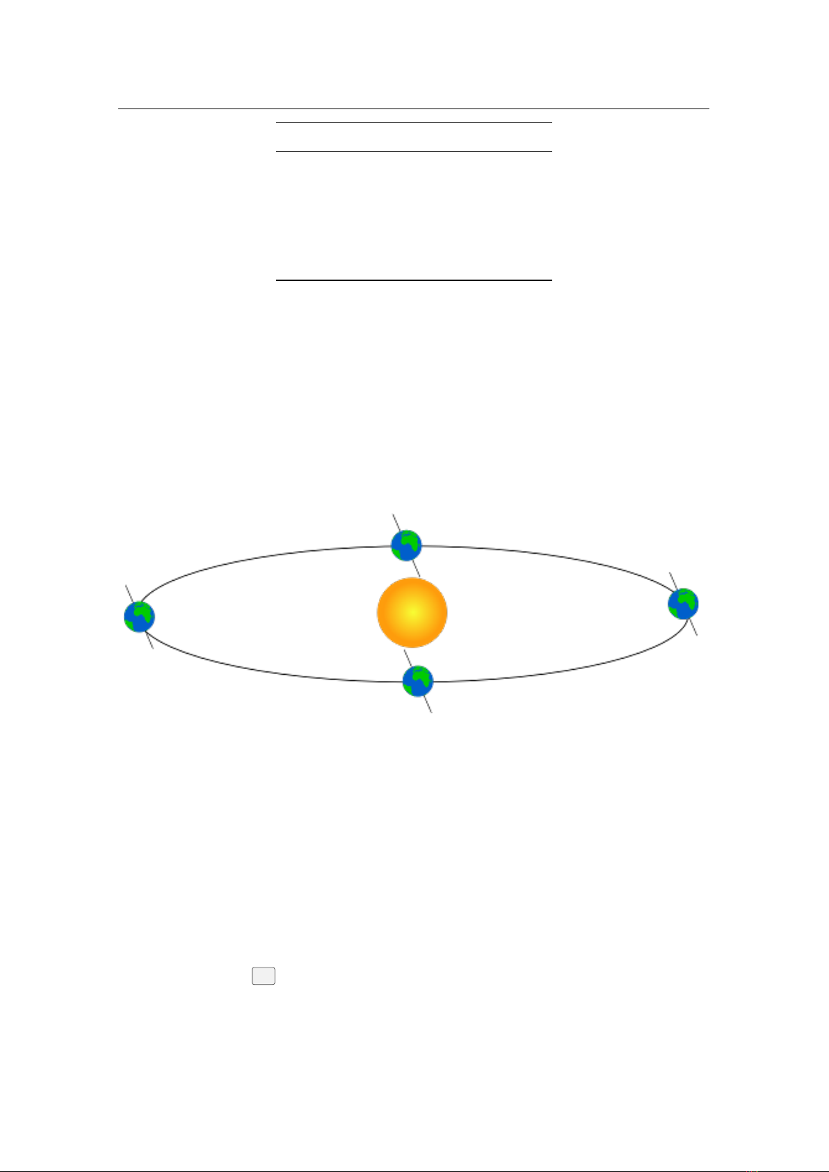
18.5 Angles 271
2015). The solution was updated in “Addendum 2020 to ‘Measurement of the Earth’s rotation: 720
BC to AD 2015’” (Morrison, F. R. Stephenson, et al., 2021). Recommended range of usage: between
years -720.0 and 2019.0 ˙n = −25.82
′′
cy
2
.
Espenak & Meeus (2006, 2014).
This solution by F. Espenak and J. Meeus, based on Morrison and F. R.
Stephenson (2004) and a polynomial fit through tabulated values for 1600-2000, is used for the NASA
Eclipse Web Site
9
, in their Five Millennium Canon of Solar Eclipses: -1900 to +3000 (Espenak
and Meeus, 2006) and Thousand Year Canon of Solar Eclipses 1501 to 2500 (Espenak, 2014). This
formula is also used in the solar, lunar and planetary ephemeris program SOLEX. Valid range of usage:
between years -1999 and 3000. ˙n = −25.858
′′
cy
2
.
Modified Espenak & Meeus (2006, 2014, 2023).
This solution
10
is a modification from Espenak & Meeus
(2006, 2014). Values for 2015-2033 are interpolated from observations and predictions by IERS
Rapid Service/Prediction Center. A simple formula is used to connect with F. Espenak’s predicted
value at year 2050. Valid range of usage: between years -1999 and 3000. ˙n = −25.858
′′
cy
2
.
Reijs (2006).
From the Length of Day (LOD; as determined by Morrison and F. R. Stephenson (2004)),
Victor Reijs derived a
∆T
formula by using a Simplex optimization with a cosine and square function.
This is based on a possible periodicity described by Morrison and F. R. Stephenson (2004). Valid
range of usage: between years -1500 and 1100. ˙n = −26.0
′′
cy
2
.
Banjevic (2006).
This solution is based on F. R. Stephenson and Morrison (1984) and was published in
“Ancient eclipses and dating the fall of Babylon” (Banjevic, 2006). Valid range of usage: between
years -2020 and 1620, with zero values outside this range. ˙n = −26.0
′′
cy
2
.
Islam, Sadiq & Qureshi (2008, 2013).
This solution by S. Islam, M. Sadiq and M. S. Qureshi, based on
Meeus and Simons (2000), was published in “Error Minimization of Polynomial Approximation of
Delta T” (Islam, Sadiq, and Qureshi, 2008) and revisited by Sana Islam in 2013. Valid range of usage:
between years 1620 and 2007, with zero values outside this range.
Khalid, Sultana & Zaidi (2014).
This polynomial approximation with 0.6 seconds of accuracy was pub-
lished in “Delta T: Polynomial Approximation of Time Period 1620–2013” (Khalid, Sultana, and
Zaidi, 2014). Valid range of usage: between years 1620 and 2013, with zero values outside this range.
Henriksson (2017).
A solution which combines Schoch’s 1931 solution (parabolic fit) with a discussion of
and correction for relativistic effects. The author claims an accurate fit for solar eclipses probably
depicted in artifacts going back to the mid-fourth millennium BC. Also with this setting, the exact
times from his paper (Henriksson, 2017) cannot be reproduced probably because the author used a
different ephemeris, but the phenomena are plausibly reproduced. Recommended range of usage:
between years -4000.0 and 2000.0 ˙n = −30.128
′′
cy
2
.
Custom equation of ∆T .
This is the quadratic formula 18.3 for calculation of
∆T
with coefficients defined
by the user.
18.5 Angles
Astronomers typically use degrees to measure angles. Since many observations require very precise
measurement, the degree is subdivided into sixty minutes of arc also known as arc-minutes. Each minute of
arc is further subdivided into sixty seconds of arc, or arc-seconds. Thus one degree is equal to 3600 seconds
of arc. Finer grades of precision are usually expressed using the SI prefixes with arc-seconds, e.g. milli
arc-seconds (one milli arc-second is one thousandth of an arc-second).
18.5.1 Notation
Degrees are denoted using the ° symbol after a number. Minutes of arc are denoted with a
′
, and seconds of
arc are denoted using
′′
. Angles are frequently given in two formats:
1.
DMS format — degrees, minutes and seconds. For example
90
°
15
′
12
′′
. When more precision is
required, the seconds component may include a decimal part, for example 90°15
′
12.432
′′
.
2. Decimal degrees, for example 90.2533°
18.5.2 Handy Angles
Being able to estimate angular distance can be very useful when trying to find objects from star maps in the
sky. One way to do this with a device called a crossbow.
9
https://eclipse.gsfc.nasa.gov/eclipse.html
10
This solution is used by default.
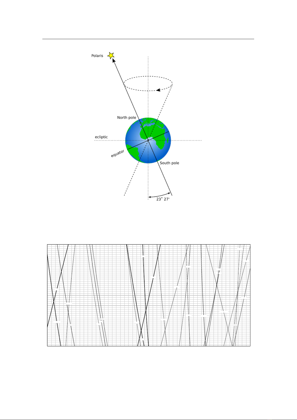
272 Chapter 18. Astronomical Concepts
Crossbows are a nice way get an idea of angular distances, but carrying one about is a little cumbersome.
A more convenient alternative is to hold up an object such as a pencil at arm’s length. If you know the length
of the pencil,
d
, and the distance of it from your eye,
D
, you can calculate its angular size,
θ
using this
formula:
θ = 2 ⋅ arctan
d
2⋅ D
(18.5)
Another, more handy (ahem!) method is to use the size of your hand at arm’s length:
Tip of little finger About 1°
Middle three fingers About 4°
Across the knuckles of the fist About 10°
Open hand About 18°
Using your hand in this way is not very precise, but it’s close enough to give you some way to translate
an idea like “Mars will be
45
° above the southeastern horizon at 21:30”. Of course, there are variations from
person to person, but the variation is compensated for somewhat by the fact that people with long arms tend
to have larger hands. In exercise 21.2 you will work out your own “handy angles”.
18.6 The Magnitude Scale
When astronomers talk about magnitude, they are referring to the brightness of an object. How bright
an object appears to be depends on how much light it is giving out and how far it is from the observer.
Astronomers separate these factors by using two measures: absolute magnitude (Mag or
M
) which is a
measure of how much light is being given out by an object, and apparent magnitude (mag or
m
) which is
how bright something appears to be in the sky.
For example, consider two 100 watt lamps, one which is a few meters away, and one which is a kilometer
away. Both give out the same amount of light – they have the same absolute magnitude. However the
nearby lamp seems much brighter – it has a much greater apparent magnitude. When astronomers talk about
magnitude without specifying whether they mean apparent or absolute magnitude, they are usually referring
to apparent magnitude.
The magnitude scale has its roots in antiquity. The Greek astronomer HIPPARCHUS defined the brightest
stars in the sky to be first magnitude, and the dimmest visible to the naked eye to be sixth magnitude. In
the 19th century British astronomer NORMAN POGSON (1829–1891) quantified the scale more precisely,
defining it as a logarithmic scale where a magnitude 1 object is 100 times as bright as a magnitude 6 object
(a difference of five magnitudes). The zero-point of the modern scale was originally defined as the brightness
of the star Vega, however this was re-defined more formally in 1982 (Aller et al., 1989). Objects brighter
than Vega are given negative magnitudes.
The absolute magnitude of a star is defined as the magnitude a star would appear if it were 10 parsecs
from the observer.
Table 18.1 lists several objects that may be seen in the sky, their apparent magnitude and their absolute
magnitude where applicable (only stars have an absolute magnitude value. Planets nor Moon emit light like
a star does – they reflect the light from the Sun).
Object m M
The Sun -27 4.8
Vega 0.05 0.6
Betelgeuse 0.47 -7.2
Sirius (the brightest star) -1.5 1.4
Venus (at brightest) -4.4 —
Full Moon (at brightest) -12.6 —
Table 18.1: Magnitudes of a few objects

18.7 Luminosity 273
18.7 Luminosity
Luminosity is an expression of the total energy radiated by a star. It may be measured in watts, however,
astronomers tend to use another expression — solar luminosities where an object with twice the Sun’s
luminosity is considered to have two solar luminosities and so on. Luminosity is related to absolute
magnitude.
18.8 Precession
Figure 18.4: Ecliptic obliquity
As the Earth orbits the Sun throughout the year, the axis of rotation (the line running through the rotational
poles of the Earth) seems to point towards the same position on the celestial sphere, as can be seen in
figure 18.4. The angle between the axis of rotation and the perpendicular of the orbital plane is called the
obliquity of the ecliptic. It is currently about
23
°
27
′
and is the angle between equatorial plane (18.2.2) and
ecliptical plane (18.2.4).
Observed over very long periods of time the direction the axis of rotation points to does actually change.
The angle between the axis of rotation and the orbital plane stays fairly constant, but the direction the axis
points — the position of the celestial pole — transcribes a figure similar to a circle on the celestial sphere.
The motion is similar to the way in which a gyroscope slowly twists, as figure 18.5 illustrates. This process
is called precession. The circles can be shown in Stellarium: from the View menu (
F4
), tab “Markings”,
switch on “Precession Circles” (4.4.4).
Precession is a slow process. The axis of rotation twists through a full
360
° about once every 26,000
years. However, over these long times other gravitational perturbations (“planetary precession”) play a role,
and what may be thought of as rigid “precession circle” can actually only show the instantaneous (current)
state. Over millennia the circle slightly varies.
Precession has some important implications:
1.
RA/Dec coordinates change over time, albeit slowly. Measurements of the positions of stars recorded
using RA/Dec coordinates must also include a date (“equinox”) for those coordinates. Therefore the
current star catalogues list their objects for the epoch and equinox J2000.0.
2.
Polaris, the Pole Star, won’t stay a good indicator of the location of the Northern Celestial Pole. In
14,000 years time Polaris will be nearly 47° away from the celestial pole!
3.
The change in declination causes a shift in the rising and setting positions of the stars along the
horizon. Figure 18.6 shows part of the horizon for latitude
ϕ = 30
° north. For a given year (left vertical
labels), make a horizontal line to find rising azimuth of the bright stars indicated by the twisting lines.
Depending on where on the celestial sphere a star is located, it may appear to move north or south, or
be almost stationary for several centuries.
18.9 Parallax
Parallax is the change of angular position of two stationary points relative to each other as seen by an
observer, due to the motion of said observer. Or more simply put, it is the apparent shift of an object against
a background due to a change in observer position.
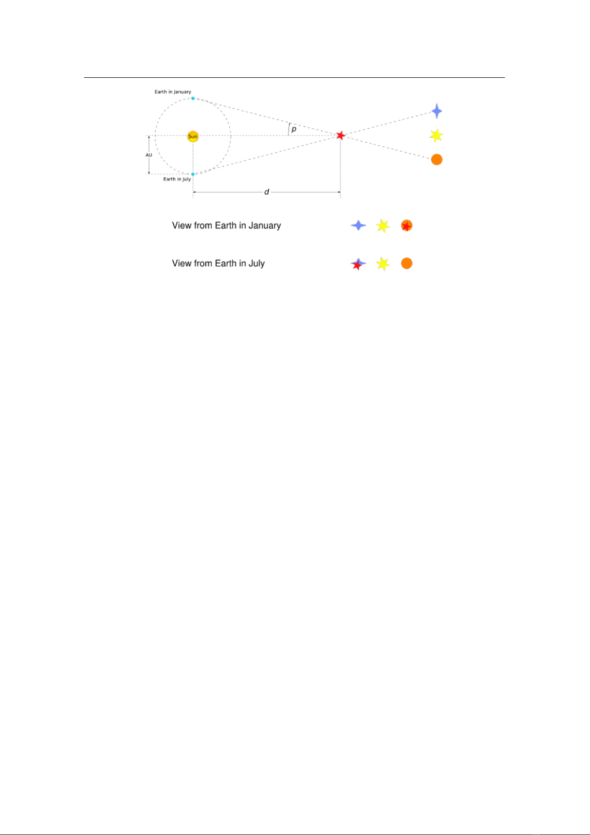
274 Chapter 18. Astronomical Concepts
Figure 18.5: Precession
90 95 100 105 110 115 120 125 130 135
85 90 95 100 105 110 115 120 125 130 135
Azimuth
-1000
-900
-800
-700
-600
-500
-400
-300
-200
-100
0
Deneb Kaitos
Rigel
Gam Ori
Mintaka
Alnilam
Alnitak
Kap Ori
Betelgeuse
Bet CMa
Sirius
Eps CMa
Del CMa
Zet Pup
Lam Vel
Alphard
Gam Cen
Spica
The Cen
Antares
Lam Sco
The Sco
Eps Sgr
Sig Sgr
Precession Shift of Stars on the Horizon
Geograpical Latitude: 30°0’ 0’’. Stars to mag=2.25. Azimuths from North, without refraction.
© Georg Zotti 2010, http://astrosim.univie.ac.at
Figure 18.6: Precession: Change of rising positions of the stars along the eastern horizon from
azimuths 85 to 135 degrees, between years 1000 BC and 0, for latitude ϕ = 30°.

18.9 Parallax 275
Figure 18.7: Stellar Parallax
This can be demonstrated by holding one’s thumb up at arm’s length. Closing one eye, note the position
of the thumb against the background. After swapping which eye is open (without moving), the thumb appears
to be in a different position against the background.
18.9.1 Geocentric and Topocentric Observations
When computing planetary positions was done manually by adding numbers tabulated in yearly almanacs,
computing the Earth’s position and, say, the position of a minor planet was usually good enough to find
the object in the sky. In both cases, the exact numbers refer to the gravitational centers of the respective
bodies. However, we are sitting on Earth’s surface, so the observed planet will be seen in a slightly shifted
location. The amount for objects in the inner solar system is usually just a few arc-seconds and is mostly
negligible when we just want to find an object. But it makes a difference when it comes to observations of
stellar occultations by planets or asteroids. Such a body may measure only a few tens of kilometers, and the
shadow track which it leaves on Earth’s surface is of approximately the same size.
11
A much closer and bigger object is the Moon, which can also occult stars. It can even occult the one big
star we call the Sun: this is a solar eclipse. And here it makes a huge difference where on the planet you are
located.
If you are interested in astronomical computing, you may still be interested in geocentric numerical
results. From the Settings panel (
F2
), tab “Tools”, there is a checkbox for “Topocentric Coordinates”.
Switch it off to put yourself into the center of the planet you are located.
18.9.2 Stellar Parallax
A similar thing happens due to the Earth’s motion around the Sun. Nearby stars appear to move against more
distant background stars, as illustrated in figure 18.7. The movement of nearby stars against the background
is called stellar parallax, or annual parallax.
Since we know the radius of the Earth’s orbit around the Sun from other methods, we can use simple
geometry to calculate the distance of the nearby star if we measure annual parallax.
As can be seen from figure 18.7, the annual parallax
p
is half the angular distance between the apparent
positions of the nearby star. The distance of the nearby object is
d
. Astronomers use a unit of distance called
the parsec (pc) which is defined as the distance at which a nearby star has p = 1
′′
.
Even the nearest stars exhibit very small movement due to parallax. The closest star to the Earth other
than the Sun is Proxima Centauri. It has an annual parallax of
0.77199
′′
, corresponding to a distance of
1.295pc
(4.22 light years). Currently, Gaia satellite is the most accurate instrument for measuring stellar
parallax. It can measure parallax at the precision level of sub milli-arcseconds for bright stars (
G < 15
),
measuring distance with ≈ 10% to stars up to 10,000 parsecs.
In Stellarium, the annual parallax can be listed in the object information for stars when available and is
11
Unfortunately Stellarium (as of v0.15.0) is not accurate enough to reliably compute such occultations. Even a
deviation of 0.5 arc-seconds is too much here.

276 Chapter 18. Astronomical Concepts
accounted for by default in the positional calculations on any Solar System objects including the Earth. You
can also exaggerate the parallax effect up to 10, 000× to make it more apparent.
18.10 Aberration of Light
When you are standing under a rainy but windless sky with an umbrella placed vertically over your head,
your feet will not be hit by raindrops. But when you are walking, raindrops which just missed the umbrella
may hit your feet. Relative to your umbrella and feet, it seems that the raindrops are coming not quite
vertically from above, but inclined from the direction you are heading into, and therefore you tilt the umbrella
slightly forward to fend off the raindrops from your feet.
Light propagates very fast compared to the motion of the planets, but still with a finite velocity. Therefore,
just like the raindrops mentioned above, light from all celestial objects seem to come in from a position
slightly distorted towards the point in space the observer is heading to.
In search for stellar parallax (see section 18.9.2), this effect of the aberration of light was fortuitously
discovered and then explained by JAMES BRADLEY (1693–1762) in 1725. This was also the final proof for
Earth’s movement around the Sun. For an observer on the moving Earth, the apparent deviation of a star
from the mean coordinates can reach
20.4”
. As the months pass, Earth is changing its direction along its
orbit, and so the light distortion also changes, i.e., the direction towards the object moves against the fixed
coordinate axes. The effect is significant when we want to compute, for example, stellar occultations by the
Moon.
In Stellarium, you can observe a slight annual wobble in all objects’ positions against the fixed celestial
grids. Just enable the equatorial grid, zoom in and run through the months. You can also exaggerate the
aberration effect up to 5× to make it more apparent.
12
18.11 Proper Motion
Proper motion is the change in the position of a star over time as a result of its motion through space relative
to the Sun. Stellarium also includes the apparent shift in position of star due to annual parallax. The star
v 25.1
exhibiting the greatest proper motion is Barnard’s Star which moves more than ten seconds of arc per year.
If you want to simulate the effect of proper motion with Stellarium, put the map into equatorial view
mode, switch off ground and cardinal marks, and set some high time lapse speed. You will see a few stars
change their locations quite soon, those are usually stars in our galactic neighbourhood (see section 21.12).
Note however some limitations:
1.
Stellarium will stop at
±100, 000
years. This limit may be still suitable for most stellar locations. The
planetary locations are not trustworthy outside of a much narrower temporal window (see section F).
You cannot simulate the sky over the dinosaurs or such things.
2.
For most bright stars (
V < 10.5
), their full 6D astrometry (2D sky positions, 2D proper motion,
parallax, radial velocity) computed by assuming straight-line motion at constant speed. Otherwise
proper motion are only modelled by linear components.
18.11.1 Binary Stars
Binary stars are listed in catalogs as two individual stars with their current proper motion which consists of a
common spatial motion and the orbital motion around their common center of gravity. Their orbital motion
around each other, where known, is now properly modelled in Stellarium.v 25.1
12
Exaggerating even more causes graphics defects and has been disabled for now.
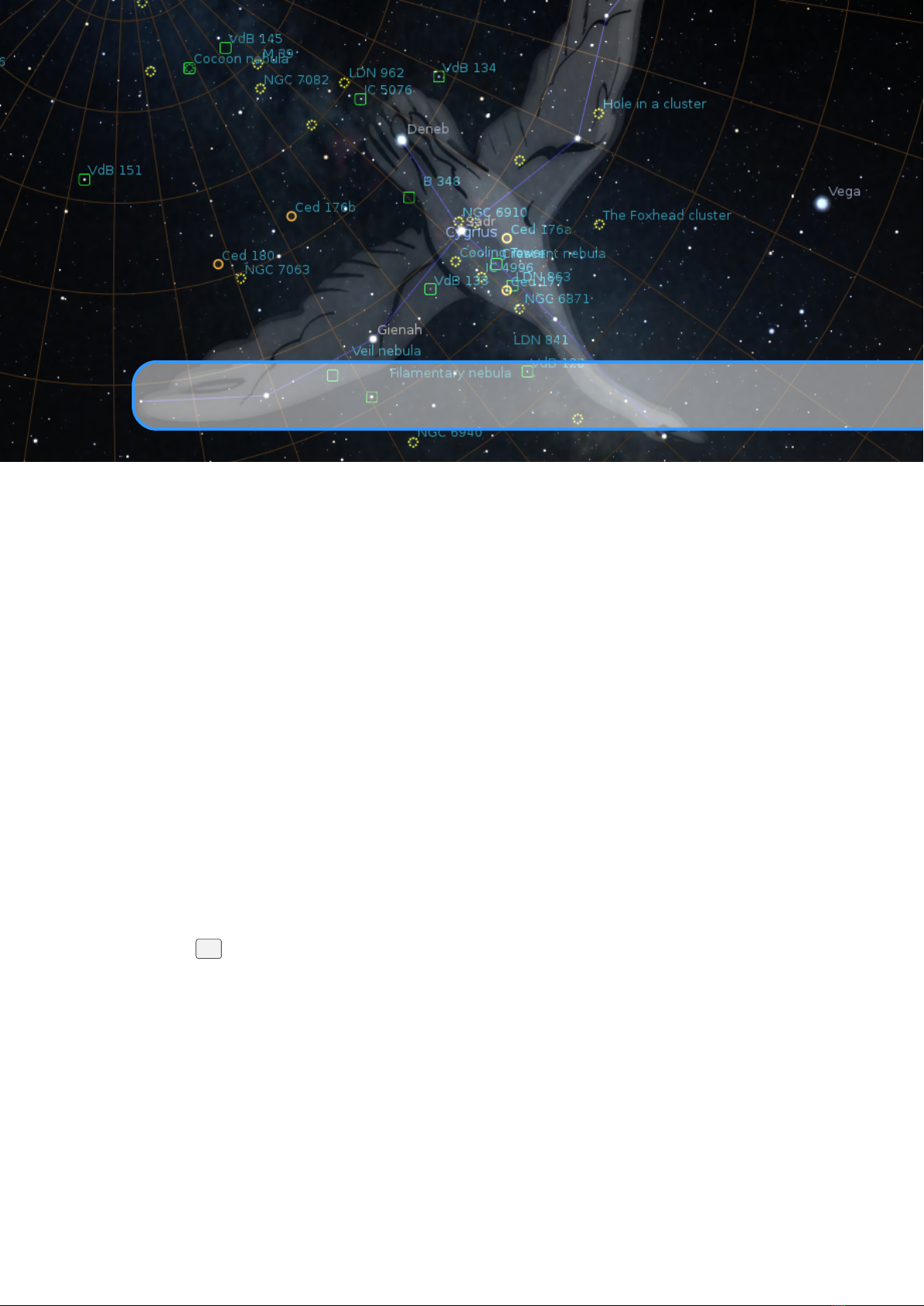
19. Astronomical Phenomena
BARRY GERDES, WITH ADDITIONS BY GEORG ZOTTI
This chapter focuses on the observational side of astronomy — what we see when we look at the sky.
19.1 The Sun
Without a doubt, the most prominent object in the sky is the Sun. The Sun is so bright that when it is in
the sky, its light is scattered by the atmosphere to such an extent that almost all other objects in the sky are
rendered invisible.
The Sun is a star like many others but it is much closer to the Earth at approximately 150 million kilome-
tres (a distance also called 1 Astronomical Unit). The next nearest star, Proxima Centauri is approximately
260,000 times further away from us than the Sun! The Sun is also known by its Latin name, Sol.
Over the course of a year, the Sun appears to move round the celestial sphere in a great circle known as
the ecliptic. Stellarium can draw the ecliptic on the sky. To toggle drawing of the ecliptic, press the
,
key.
WARNING: Looking at the Sun with even the smallest telescope or binoculars can permanently damage
the eye. Never look at the Sun without using the proper filters attached to the front end (objective lens)
of your instrument! Never use screw-in ocular filters, they may break in the heat and expose your eye to
damaging amounts of energy. By far the safest way to observe the Sun is to look at it on a computer screen,
courtesy of Stellarium!
19.1.1 Twilight
The sunlight is scattered in Earth’s atmosphere even if the Sun is below the horizon. The period after sunset
when the Sun is higher than
−6
° is called civil twilight. The sky is generally bright enough for outdoor
activity or reading the newspaper.
As time progresses, the first stars will appear. The phase where the Sun is between
−6
° and
−12
° below
the (mathematical) horizon is called nautical twilight: before the invention of satellite navigation, celestial
navigation was used to find a ship’s position on the oceans. This required that it was still bright enough so
that the horizon line was visible, but already dark enough to see enough stars to clearly identify them and
measure the altitude of a few of them. (See also section 14.7.)
The twilight phase when the Sun is between
−12
° and
−18
° is called astronomical twilight. Only the
western horizon shows some brightening, but else the natural sky is “almost” as dark as it can get.
In the morning the game is reversed. Dawn starts with astronomical twilight, progresses to nautical and
civil twilight, and sunrise ends the night.
In Stellarium, you can set the time when the Sun reaches a configured altitude. See section 4.8.1 about
how to configure the program.

278 Chapter 19. Astronomical Phenomena
Figure 19.1: Ursa Major
19.2 Stars
The Sun is just one of billions of stars. Even though many stars have a much greater absolute magnitude than
the Sun (they give out more light), they have an enormously smaller apparent magnitude due to their large
distance. Stars have a variety of forms — different sizes, brightnesses, temperatures, and colours. Measuring
the position, distance and attributes of the stars is known as astrometry, and is a major part of observational
astronomy.
19.2.1 Multiple Star Systems
Many stars have stellar companions. As many as six stars can be found orbiting one-another in close
associations known as multiple star systems — binary systems being the most common with two stars.
Multiple star systems are more common than solitary stars, putting our Sun in the minority group.
Sometimes multiple stars orbit each other in a way that means one will periodically eclipse the other.
These are eclipsing binaries or Algol variables.
19.2.1.1 Optical Doubles & Optical Multiples
Sometimes two or more stars appear to be very close to one another in the sky, but in fact have great
separation, being aligned from the point of view of the observer but of different distances. Such pairings are
known as optical doubles and optical multiples.
19.2.2 Constellations
The constellations are groupings of stars that are visually close to one another in the sky. The actual groupings
are fairly arbitrary — different cultures have grouped stars together into different constellations. In many
cultures, the various constellations have been associated with mythological entities. As such people have
often projected pictures into the skies as can be seen in figure 19.1 which shows the constellation of Ursa
Major. On the left is a picture with the image of the mythical Great Bear, on the right only a line-art version
(or stick figure) is shown.
Stellarium can draw both constellation diagrams and artistic representations of the constellations.
Multiple sky cultures are supported: Stellarium’s default ’Modern’ skyculture is an amalgamate of European
scientific traditions that are rooted in Ptolemy’s Almagest, with constellation figures mostly from ancient
Greek mythology. In the upcoming era of Islam, the Almagest was translated to Arab, including star
names that often just described the location of a star within the constellation. Around the year 1000 the
Almagest was re-introduced to Western Europe, but some star names were misspelled and transferred without
re-tranalation, introducing a large number of star names of Arab origin now in use for many centuries.
Aside from historical and mythological value still valued by storytellers around the campfires, to the
modern astronomer the constellations provide a way to segment the sky for the purposes of describing
locations of objects. Indeed, one of the first tasks for an amateur observer is astrognosis (learning the
constellations) — the process of becoming familiar with the relative positions of the constellations, at what
time of year a constellation is visible, and in which constellations observationally interesting objects reside.
As scientific astronomy evolved in the Renaissance and later, star atlases were produced, each introducing
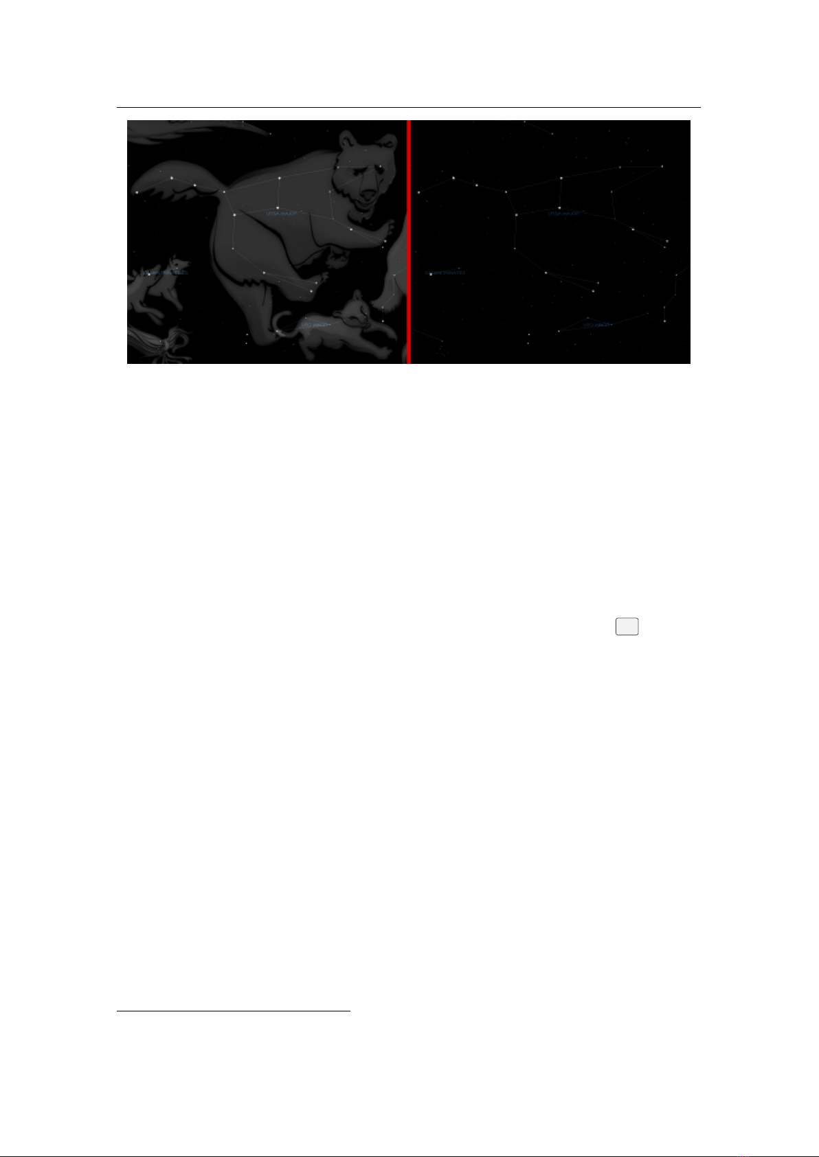
19.2 Stars 279
Abbr. Name Genitive Abbr. Name Genitive
And Andromeda Andromedae Lac Lacerta Lacertae
Ant Antlia Antliae Leo Leo Leonis
Aps Apus Apodis LMi Leo Minor Leonis Minoris
Aqr Aquarius Aquarii
Lep Lepus Leporis
Aql Aquila Aquilae Lib Libra Librae
Ara Ara Arae Lup Lupus Lupi
Ari Aries Arietis Lyn Lynx Lyncis
Aur Auriga Aurigae Lyr Lyra Lyrae
Boo Bootes Bootis Men Mensa Mensae
Cae Caelum Caeli Mic Microscopium Microscopii
Cam Camelopardalis Camelopardalis Mon Monoceros Monocerotis
Cnc Cancer Cancri Mus Musca Muscae
Cvn Canes Venatici Canum Venaticorum Nor Norma Normae
CMa Canis Maior Canis Maioris Oct Octans Octantis
CMi Canis Minor Canis Minoris
Oph Ophiuchus Ophiuchi
Cap Capricornus Capricorni Ori Orion Orionis
Car Carina Carinae Pav Pavo Pavonis
Cas Cassiopeia Cassiopeiae Peg Pegasus Pegasi
Cen Centaurus Centauri Per Perseus Persei
Cep Cepheus Cephei Phe Phoenix Phoenicis
Cet Cetus Ceti Pic Pictor Pictoris
Cha Chamaeleon Chamaeleonis Psc Pisces Piscium
Cir Circinus Circini PsA Piscis Austrinus Piscis Austrini
Col Columba Columbae Pup Puppis Puppis
Com Coma Berenices Comae Berenicis
Pyx Pyxis Pyxidis
CrA Corona Australis Coronae Australis Ret Reticulum Reticuli
CrB Corona Borealis Coronae Borealis Sge Sagitta Sagittae
Crt Crater Crateris Sgr Sagittarius Sagittarii
Crv Corvus Corvi Sco Scorpius Scorpii
Cru Crux Crucis Scl Sculptor Sculptoris
Cyg Cygnus Cygni
Sct Scutum Scuti
Del Delphinus Delphini
Ser Serpens Serpentis
Dor Dorado Doradus Sex Sextans Sextantis
Dra Draco Draconis Tau Taurus Tauri
Equ Equuleus Equulei Tel Telescopium Telescopii
Eri Eridanus Eridani
Tri Triangulum Trianguli
For Fornax Fornacis TrA Triangulum Australe Trianguli Australis
Gem Gemini Geminorum Tuc Tucana Tucanae
Gru Grus Gruis UMa Ursa Maior Ursae Maioris
Her Hercules Herculis UMi Ursa Minor Ursae Minoris
Hor Horologium Horologii Vel Vela Velae
Hya Hydra Hydrae Vir Virgo Virginis
Hyi Hydrus Hydri Vol Volans Volantis
Ind Indus Indi Vul Vulpecula Vulpeculae
Table 19.1: The official 88 IAU constellation names and abbreviations
α alpha ε epsilon ι iota ν nu ρ rho ϕ phi
β beta ζ zeta κ kappa ξ xi σ sigma χ chi
γ gamma η eta λ lambda o omicron τ tau ψ psi
δ delta θ theta µ mu π pi υ upsilon ω omega
Table 19.2: The Greek alphabet used by Bayer

280 Chapter 19. Astronomical Phenomena
more constellations to fill gaps left between the classic 48 Ptolemaic constellations, with artistic figures
often overwhelming the actual star map. The telescope age and needs to assign each fixed celestial object
coordinates and a ’host constellation’ finally had to bring an end to the uncontrolled growth of officially
recognized constellations. In 1930, the International Astronomical Union has adopted 88 constellations
as a common system for segmenting the sky (Table 19.1). Some formalisation has been adopted, each
constellation having a proper name in Latin, and a three letter abbreviation of that name. For example, Ursa
Major has the abbreviation UMa. Also, the IAU constellations have clearly defined boundaries(Delporte,
1930), which you can draw in Stellarium when you press the
B
key
1
. The IAU constellation a selected
object is placed in is also available in the object information data (Roman, 1987), regardless of the currently
active sky culture.
On the other hand, the shapes of mythological figures, and also stick figures, have not been canonized,
so you will likely find deviations between Stellarium’s default skyculture and your favourite printed atlas. In
this sense, do also not assume Stellarium’s default stick figures to be in any way authoritative. As any other,
they are an artistic interpretation that should help memorizing and discerning the constellations.
19.2.2.1 Asterisms
As nonscientific observing of the sky became a pastime for non-scientists (amateur astronomers) in the late
19th century, some easy to recognize star groups were described and labeled in sky observing guides. These
are internationally not standardized and may show even regionally differing names for (almost) the same
figure. For example, the seven bright stars of Ursa Major are widely recognised, known variously as “the
plough”, the “pan-handle”, “greater wagon” or the “big dipper”.
After the canonisation of the IAU constellations, these figures became commonly known as asterisms
2
.
In Stellarium, you can display them as stick figures with name labels in colors different from the “main”
constellations.
19.2.2.2 Non-European Constellations
Many other sky cultures are available in Stellarium which show constellations and other elements of
ethnoastronomy of other traditions, contributed by users and scientists from all over the world, and showing
the diversity and ubiquity of human interest in the sky all around the globe.
We welcome well-made contributions, but as time evolves these skyculture contributions may be further
extended by the original authors, other contributors (if allowed by respective licenses), or removed if found
problematic. See chapter 9 for full details.
19.2.3 Star Names
The brighter stars often have one or more common names relating to mythical characters from the various
traditions. For example the brightest star in the sky, Sirius, is also known as The Dog Star (the name Canis
Major — the constellation Sirius is found in — is Latin for “The Great Dog”).
Most bright names have been given names in antiquity. PTOLEMY’s most influential book, the Syntaxis,
was translated to the Arab language in the age of early Muslim scientists. When, centuries later, the
translation, called Almagest, was re-introduced to the re-awakening European science, those names, which
often only designated the position of the star within the figure, were taken from the books, often misspelled,
and used henceforth as proper names.
A few more proper names have been added later, sometimes dedicatory names added by court as-
tronomers into their maps. There are also 3 stars named after the victims of the Apollo 1 disaster in 1967.
Today, the International Astronomical Union (IAU) is the only scientifically accepted authority which can
give proper names to stars, and a ‘Working Group on Star Names’ (WGSN) has been established. Apart
from canonizing one spelling for the well-known stars and avoiding using the same name for multiple stars,
recently WGSN has started to assign star names from non-European cultures to hitherto unnamed (usually
dimmer, but still naked-eye) stars in order to diversify star names. (Constellation names and IAU borders are
not affected.) Stellarium closely follows this development in the default ‘Modern’ and ‘IAU’ Skycultures.
Some companies offer a paid name service for commemoration or dedication of a star for deceased
relatives or such, but all you get here is a piece of paper with coordinates of (usually) an unremarkably dim
star only visible in a telescope, and a name to remember, stored (at best) in the company’s database.
1
These boundaries or borders have been defined using coordinates from 1875. Due to the effect of precession, these
borders are no longer parallel to today’s coordinate grid.
2
Note that in other scientific contexts, ‘asterism’ may also be the general designation of a star figure (often of other
cultures). However, in Stellarium an ‘asterism’ can be understood as ‘informal second-class figure’ that may be used for
culture-dependent purposes.

19.2 Stars 281
There are several more formal naming conventions that are in common use.
19.2.3.1 Bayer Designation
The German astronomer JOHANN BAYER (1572–1625) devised one such system for his atlas, the Ura-
nographia, first published in 1603. His scheme names the stars according to the constellation in which they
lie prefixed by a lower case Greek letter (see Tab. 19.2), starting at
α
for (usually) the brightest star in the
constellation and proceeding with β , γ, . . . in descending order of apparent magnitude. For example, such a
Bayer Designation for Sirius is “
α
Canis Majoris” (note that the genitive form of the constellation name
is used, refer to Table 19.1; today also the short form
α
CMa is in use). There are some exceptions to the
descending magnitude ordering, and some multiple stars (both real and optical) are named with a numerical
superscript after the Greek letter, e.g. π
1
...
π
6
Orionis.
19.2.3.2 Flamsteed Designation
English astronomer JOHN FLAMSTEED (1646–1719) numbered stars in each constellation in order of
increasing right ascension followed by the genitive form of the constellation name, for example “61 Cygni”
(or short: “61 Cyg”).
19.2.3.3 Hipparcos
Hipparcos (for High Precision Parallax Collecting Satellite) was an astrometry mission of the European
Space Agency (ESA) dedicated to the measurement of stellar parallax and the proper motions of stars. The
project was named in honour of the Greek astronomer HIPPARCHUS.
Ideas for such a mission dated from 1967, with the mission accepted by ESA in 1980. The satellite was
launched by an Ariane 4 on 8 August 1989. The original goal was to place the satellite in a geostationary
orbit above the earth, however a booster rocket failure resulted in a highly elliptical orbit from 500 to
35,800 km (310 to 22,240 miles) altitude. Despite this difficulty, all of the scientific goals were accomplished.
Communications were terminated on 15 August 1993.
The program was divided in two parts: the Hipparcos experiment whose goal was to measure the five
astrometric parameters of some 120,000 stars to a precision of some 2 to 4 milli arc-seconds and the Tycho
experiment, whose goal was the measurement of the astrometric and two-colour photometric properties of
some 400,000 additional stars to a somewhat lower precision.
The final Hipparcos Catalogue (120,000 stars with 1 milli arc-second level astrometry) and the final
Tycho Catalogue (more than one million stars with 20-30 milli arc-second astrometry and two-colour
photometry) were completed in August 1996. The catalogues were published by ESA in June 1997. The
Hipparcos and Tycho data have been used to create the Millennium Star Atlas: an all-sky atlas of one million
stars to visual magnitude 11, from the Hipparcos and Tycho Catalogues and 10,000 non-stellar objects
included to complement the catalogue data.
Figure 19.2: Star Names and Data
There were questions over whether Hipparcos has a systematic error of about 1 milli arc-second in at
least some parts of the sky. The value determined by Hipparcos for the distance to the Pleiades is about 10%
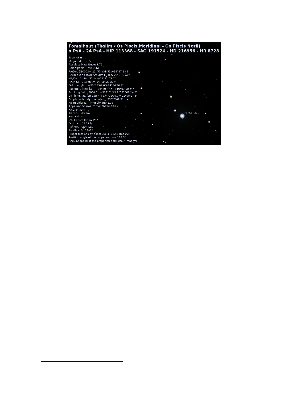
282 Chapter 19. Astronomical Phenomena
Spectral Type Surface Temperature (K) Star Colour
O 28,000—50,000 Blue
B 10,000—28,000 Blue-white
A 7,500—10,000 White-blue
F 6,000—7,500 Yellow-white
G 4,900—6,000 Yellow
K 3,500—4,900 Orange
M 2,000—3,500 Red
Table 19.3: Spectral Types
less than the value obtained by some other methods. By early 2004, the controversy remained unresolved.
Stellarium uses the Hipparcos Catalogue for star data, as well as having traditional names for many of
the brighter stars. The stars tab of the search window allows for searching based on a Hipparcos Catalogue
number (as well as traditional names), e.g. the star Sadalmelik in the constellation of Aquarius can be found
by searching for the name, or its Hipparcos number, 109074.
Figure 19.2 shows the information Stellarium displays when a star is selected. At the top, the common
name, Bayer/Flamsteed designations and Hipparcos number are shown, followed by the RA/Dec coordinates,
apparent magnitude, distance and other data.
19.2.4 Spectral Type & Luminosity Class
Stars have many different colours. Seen with the naked eye most appear to be white, but this is due to the
response of the eye — at low light levels the eye is not sensitive to colour. Typically the unaided eye can
start to see differences in colour only for stars that have apparent magnitude brighter than 1. Betelgeuse, for
example has a distinctly red tinge to it, and Sirius appears to be blue, while Vega is the prototype “white”
star.
By splitting the light from a star using a prism attached to a telescope and measuring the relative
intensities of the colours of light the star emits — the spectrum — a great deal of interesting information
can be discovered about a star including its surface temperature, and the presence of various elements in its
atmosphere.
Astronomers groups stars with similar spectra into spectral types, denoted by one of the following letters:
O, B, A, F, G, K and M.
3
Type O stars have a high surface temperature (up to around 50,000 K) while the at
other end of the scale, the M stars are red and have a much cooler surface temperature, typically 3000 K. The
Sun is a type G star with a surface temperature of around 5,500 K. Spectral types may be further sub-divided
using a numerical suffix ranging from 0-9 where 0 is the hottest and 9 is the coolest. Table 19.3 shows the
details of the various spectral types.
For about 90% of stars, the absolute magnitude increases as the spectral type tends to the O (hot) end of
the scale. Thus the whiter, hotter stars tend to have a greater luminosity. These stars are called main sequence
stars. There are however a number of stars that have spectral type at the M end of the scale, and yet they
have a high absolute magnitude. These stars are close to the ends of their lives and have a very large size,
and consequently are known as giants, the largest of these known as super-giants.
There are also stars whose absolute magnitude is very low regardless of the spectral class. These are
known as dwarf stars, among them white dwarfs (dying stars) and brown dwarfs (“failed stars”).
The luminosity class is an indication of the type of star — whether it is main sequence, a giant or a
dwarf. Luminosity classes are denoted by a number in roman numerals, as described in table 19.4.
Plotting the luminosity of stars against their spectral type/surface temperature gives a diagram called a
Hertzsprung-Russell diagram (after the two astronomers EJNAR HERTZSPRUNG (1873–1967) and HENRY
NORRIS RUSSELL (1877–1957) who devised it). A slight variation of this is shown in figure 19.3 (which is
technically a colour/magnitude plot).
19.2.5 Variable Stars
Most stars are of nearly constant luminosity. The Sun is a good example of one which goes through relatively
little variation in brightness (usually about 0.1% over an 11 year solar cycle). Many stars, however, undergo
3
The classic mnemonic for students of astrophysics says: “Oh, Be A Fine Girl, Kiss Me”.

19.2 Stars 283
Figure 19.3: Hertzsprung-Russell Diagram
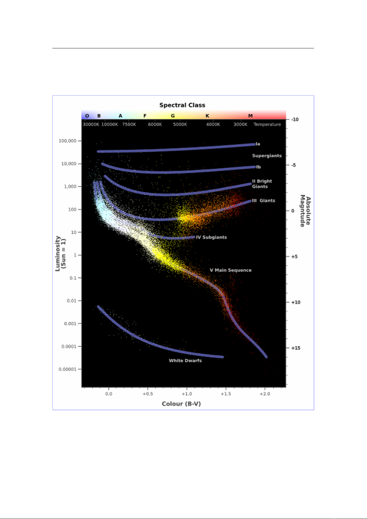
284 Chapter 19. Astronomical Phenomena
Luminosity class Description
Ia, Ib Super-giants
II Bright giants
III Normal giants
IV Sub-giants
V Main sequence
VI Sub-dwarfs
VII White-dwarfs
Table 19.4: Luminosity Classification
New Moon
The moon’s disc is fully in shadow, or there is just a slither of illuminated surface on
the edge.
Waxing Crescent
Less than half the disc is illuminated, but more is illuminated each night.
First Quarter
Approximately half the disc is illuminated, and increasing each night.
Waxing Gibbous
More than half of the disc is illuminated, and still increasing each night.
Full Moon
The whole disc of the moon is illuminated.
Waning Gibbous
More than half of the disc is illuminated, but the amount gets smaller each night.
Last Quarter
Approximately half the disc is illuminated, but this gets less each night.
Waning Crescent
Less than half the disc of the moon is illuminated, and this gets less each night.
Table 19.5: Lunar Phases
significant variations in luminosity, and these are known as variable stars. There are many types of variable
stars falling into two categories, intrinsic and extrinsic.
Intrinsic variables are stars which have intrinsic variations in brightness, that is, the star itself gets
brighter and dimmer. There are several types of intrinsic variables, probably the best-known and most
important of which is the Cepheid variable whose luminosity is related to the period with which its brightness
varies. Since the luminosity (and therefore absolute magnitude) can be calculated, Cepheid variables may be
used to determine the distance of the star when the annual parallax is too small to be a reliable guide. This is
especially welcome because they are giant stars, and so they are even visible in neighboring galaxies.
Extrinsic variables are stars of constant brightness that show changes in brightness as seen from the
Earth. These include rotating variables, stars whose apparent brightness change due to rotation, and eclipsing
binaries.
Stellarium’s catalogs include many kinds variable stars. See section C.3 for more details.
19.3 Our Moon
The Moon is the large satellite which orbits the Earth approximately every 28 days. It is seen as a large bright
disc in the early night sky that rises later each day and changes shape into a crescent until it disappears near
the Sun. After this it rises during the day then gets larger until it again becomes a large bright disc again.
19.3.1 Phases of the Moon
As the moon moves round its orbit, the amount that is illuminated by the sun as seen from a vantage point on
Earth changes. The result of this is that approximately once per orbit, the moon’s face gradually changes
from being totally in shadow to being fully illuminated and back to being in shadow again. This process is
divided up into various phases as described in table 19.5.
19.3.2 The Lunar Magnitude
The eastern half of the Moon has more dark maria, therefore careful studies (Russell, 1916) have shown
that in the waxing phases the Moon is slightly brighter than in the waning phase of the same degree of
illumination.
Around Full Moon, the Moon shows an opposition surge, a strong increase in brightness which Krisciunas
and B. Schaefer (1991) describe as a 35% increase in luminous flux over the curve extrapolated from
measurements when the phase angle α< 7
○
.

19.4 The Major Planets 285
Figure 19.4: The Planets
Of course, just at Full Moon when the opposition is near-perfect, the Moon will also move through
Earth’s shadow during a Lunar eclipse.
The Moon reflects not only sunlight which directly hits it, but also sunlight reflected from Earth to the
Moon (Agrawal, 2016). This earthshine, also known as ashen glow, is brightest when the Moon is most
strongly illuminated by the Earth, i.e., when the Moon as seen from Earth shows only a thin crescent. In these
days around the New Moon, the thin crescent can often be seen complemented into a softly glowing full disk.
Stellarium’s estimate for visual magnitude is based on the mentioned references and a new standard value
for the solar illumination constant of 133.1 klx (Ashdown, 2019).
19.4 The Major Planets
Unlike the stars whose relative positions remain more or less constant, the planets seem to move across the
sky over time (the word “planet” comes from the Greek for “wanderer”). The planets are siblings of the
Earth, massive bodies that are in orbit around the Sun. Until 2006 there was no formal definition of a planet,
leading to some confusion about the classification for some bodies traditionally regarded as being planets,
but which didn’t seem to fit with the others.
In 2006 the International Astronomical Union (IAU) defined a planet as a celestial body that, within the
Solar System:
1. is in orbit around the Sun
2.
has sufficient mass for its self-gravity to overcome rigid body forces so that it assumes a hydrostatic
equilibrium (nearly round) shape; and
3. has cleared the neighbourhood around its orbit
or within another system:
1. is in orbit around a star or stellar remnants
2. has a mass below the limiting mass for thermonuclear fusion of deuterium; and
3. is above the minimum mass/size requirement for planetary status in the Solar System.
Moving from the Sun outwards, the 8 major planets are: Mercury, Venus, Earth, Mars, Jupiter, Saturn,
Uranus and Neptune. Since the formal definition of a planet in 2006 Pluto has been relegated to having the
status of dwarf planet, along with bodies such as Ceres and Eris. See figure 19.4.
19.4.1 Terrestrial Planets
The planets closest to the sun are called collectively the terrestrial planets. The terrestrial planets are:
Mercury, Venus, Earth and Mars.
The terrestrial planets are relatively small, comparatively dense, and have solid rocky surface. Most of
their mass is made from solid matter, which is mostly rocky and/or metallic in nature.
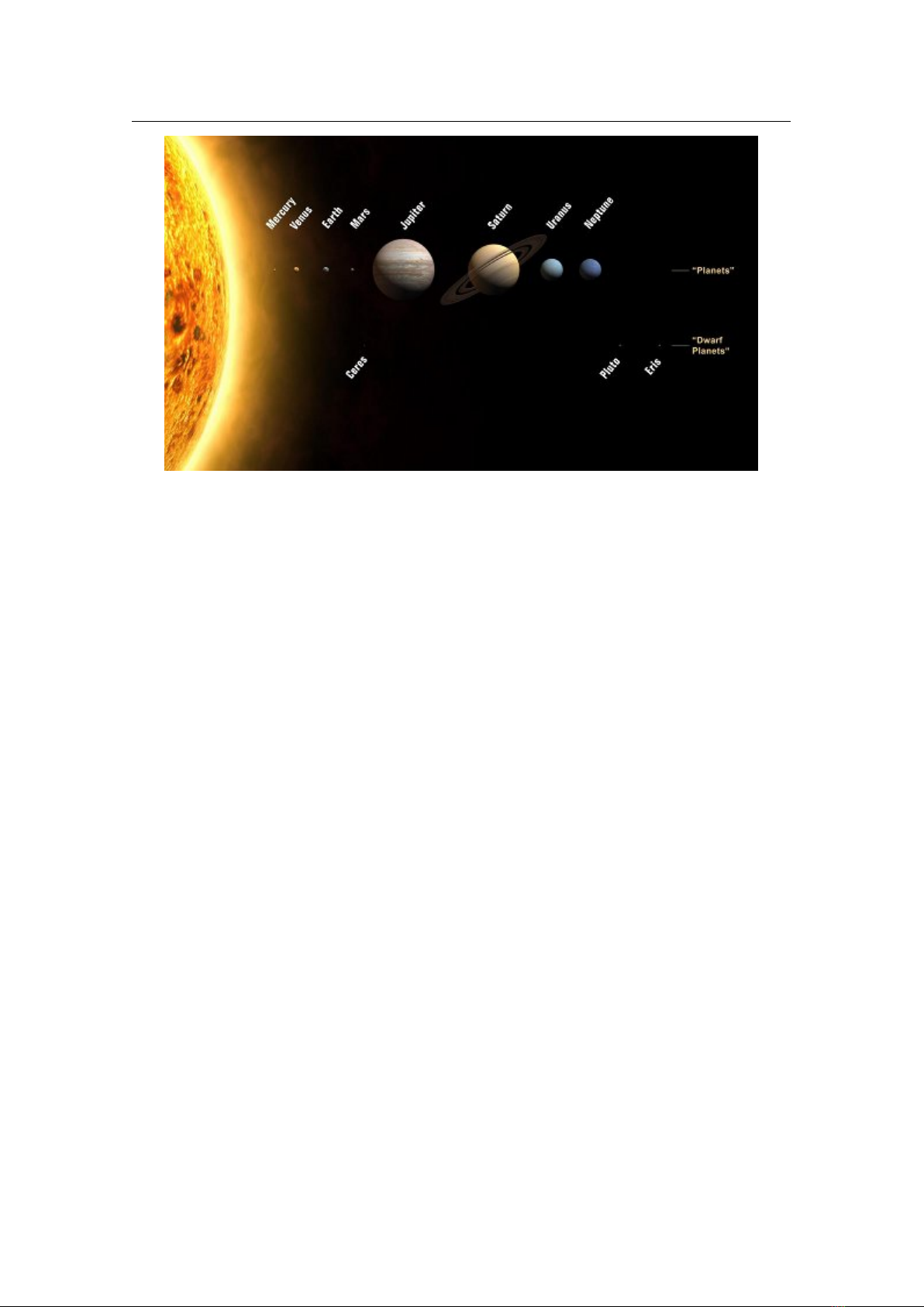
286 Chapter 19. Astronomical Phenomena
19.4.2 Jovian Planets
Jupiter, Saturn, Uranus and Neptune make up the Jovian planets, also called gas giants. They are much more
massive than the terrestrial planets, and do not have a solid surface. Jupiter is the largest of all the planets
with a diameter of about 12, and mass over 300 times that of the Earth!
The Jovian planets do not have a solid surface – the vast majority of their mass being in gaseous form
(although they may have rocky or metallic cores). Because of this, they have an average density which is
much less than the terrestrial planets. Saturn’s mean density is only about
0.7gcm
3
– it would float in water!
19.4.3 Apparent Magnitudes of the Planets
The apparent magnitude of the planets can be found in astronomical almanachs. Over time, several scientific
studies have refined these models. A few of them have been implemented in Stellarium:
Müller 1893
G. Müller formulated visual magnitudes for the planets from visual observations of 1877–1891.
They can be found in Meeus (1998) and Wilkins (1961). They give notably lower brightness estimates
than the later models, which however provide instrumental magnitudes in the Johnson V photometric
system. Several important historical studies from the early 20th century are based on these estimates.
Astronomical Almanac 1984
This model was used in the Astronomical Almanac starting in 1984. The
expressions are allegedly “due to D. L. Harris”, but J. Meeus (1998, p.286) denies this origin.
Explanatory Supplement 1992 Expressions from Seidelmann (1992).
Explanatory Supplement 2013 Expressions from Urban and Seidelmann (2013).
Mallama & Hilton 2018
The currently most modern expressions include e.g. a model for Mars which takes
the brightening and dimming of albedo features into account (Mallama and J. L. Hilton, 2018).
Generic A simple model based on albedo, size and distance.
19.5 The Minor Bodies
As well as the Major Planets, the Solar system also contains innumerable smaller bodies in orbit around
the Sun. These are generally the dwarf planets (Ceres, Pluto, Eris), the other minor planets, also known as
planetoids or asteroids, and comets.
While the positions of the major planets can meanwhile be computed for many millennia in the past and
future, the minor bodies have only been systematically observed since the beginning of the 19th century.
4
The small masses occasionally pass by the larger planets which exert gravitational forces, so that the orbits
of the minor bodies are not stable and cannot be computed for long periods. The positions are computed by
using osculating orbital elements, which describe the motions on instantaneous Kepler orbits
5
. If you want
to compute positions of these objects with Stellarium, you need to have valid (current) orbital elements. See
Solar System Editor plugin (section 13.11) and Appendix D.2.2 for more details. For long-term valid orbital
data, see Appendix D.2.4.
19.5.1 Asteroids
Asteroids are celestial bodies orbiting the Sun in more or less regular orbits mostly between Mars and Jupiter.
They are generally rocky bodies like the inner (terrestrial) planets, but of much smaller size. They are
countless in number ranging in size from about ten meters to hundreds of kilometres.
19.5.2 Comets
A comet is a small body in the Solar system that orbits the Sun and (at least occasionally) exhibits a coma
(or atmosphere) and/or a tail.
Most comets have a very eccentric orbit (featuring a highly flattened ellipse, or even a parabolic track),
and as such spend most of their time a very long way from the Sun. Comets are composed of rock, dust and
ices. When they come close to the Sun, the heat evaporates the ices, causing a gaseous release. This gas and
loose material which comes away from the body of the comet is swept away from the Sun by the Solar wind,
forming the tail. The outgassing may also change the orbit of the comet, so that its orbital elements should
be used only for a few months around their epoch.
Most larger comets exhibit two kinds of tail: a straight gas tail (often blue-green in photographs), and a
wider, occasionally curved dust tail (reflecting whitish sunlight).
4
The first discovered asteroid, (1) Ceres, was in fact discovered on January 1, 1801.
5
The mathematician and astronomer JOHANN ES KEPLER (1571–1630) discovered that planets do not move on
circles (which had been postulated since antiquity), but on “conical sections”, i.e., ellipses, parabolae or even hyperbolae.
The latter two can be observed for far-out comets and recently even interstellar objects passing the Sun.

19.6 Meteoroids 287
Comets whose orbit brings them close to the Sun more frequently than every 200 years are considered
to be short period comets, the most famous of which is probably Comet Halley, named after the British
astronomer EDMUND HALLEY (1656–1741/42
6
), which has an orbital period of roughly 76 years.
19.6 Meteoroids
These objects are small pieces of space debris left over from the early days of the Solar system or which
crumbled off a comet when it came close to the sun. These particles orbit the Sun and come in a variety of
shapes, sizes an compositions, ranging from microscopic dust particles up to about ten meters across.
Sometimes these objects collide with the Earth. The closing speed of these collisions is generally
extremely high (tens of kilometres per second). When such an object ploughs through the Earth’s atmosphere,
a large amount of kinetic energy is converted into heat and light, and a visible flash or streak can often be
seen with the naked eye. Even the smallest particles can cause these events which are commonly known as
shooting stars.
While smaller objects tend to burn up in the atmosphere, larger, denser objects can penetrate the
atmosphere and strike the surface of the planet, sometimes leaving meteor craters.
Sometimes the angle of the collision means that larger objects pass through the atmosphere but do not
strike the Earth. When this happens, spectacular fireballs are sometimes seen.
To clarify some terminology:
Meteoroids are the objects when they are floating in space.
Meteor is the name given to the visible atmospheric phenomenon.
Shooting Star colloquial term for a small meteor
Fireball, Bolide
term for a very bright meteor. These illuminate the landscape, sometimes for several
seconds, and occasionally even cause sounds. These are also candidates for
Meteorites , the objects that penetrate the atmosphere and land (or impact) on the surface.
In some nights over the year you can observe increased meteorite activity. Those meteors seem to come
from a certain point in the sky, the Radiant. But what we see is similar to driving through a mosquito swarm
which all seem to come head-on. Earth itself moves through space, and sweeps up a dense cloud of particles
which originates from a comet’s tail. Stellarium’s Meteor Shower plugin (see section 14.6) can help you
planning your next meteor observing night.
19.7 Zodiacal Light and Gegenschein
In very clear nights on the best observing sites, far away from the light pollution of our cities, you can
observe a feeble glow also known as “false twilight” after evening twilight in the west, or before dawn in the
east. The glow looks like a wedge of light along the ecliptic. Exactly opposite the sun, there is another dim
glow that can be observed with dark-adapted eyes in perfect skies: the Gegenschein (counterglow).
This is sunlight reflected off the same dust and meteoroids in the plane of our Solar system which is the
source of meteors. Stellarium’s sky can show the Zodiacal light (Kwon, Hong, and Weinberg, 2004), but
observe how quickly light pollution kills its visibility!
19.8 The Milky Way
There is a band of very dense stars running right round the sky in huge irregular stripe. Most of these stars
are very dim, but the overall effect is that on very dark clear nights we can see a large, beautiful area of
diffuse light in the sky. It is this for which we name our galaxy the Milky Way.
The reason for this effect is that our galaxy is somewhat like a disc, and we are off to one side. Thus
when we look towards the centre of the disc, we see more a great concentration of stars (there are more star
in that direction). As we look out away from the centre of the disc we see fewer stars - we are staring out
into the void between galaxies!
It’s a little hard to work out what our galaxy would look like from far away, because when we look up at
the night sky, we are seeing it from the inside. All the stars we can see are part of the Milky Way, and we can
see them in every direction. However, there is some structure. There is a higher density of stars in particular
places.
6
EDMUND HALLEY lived in a time when Great Britain still used the Julian calendar and started the years in March.
He died on January 14th, 1741 (British Julian), which was called January 25th 1742 (Gregorian) in most other European
countries.

288 Chapter 19. Astronomical Phenomena
19.9 Nebulae
Seen with the naked eye, binoculars or a small telescope, a nebula (plural nebulae) is a fuzzy patch on the
sky. Historically, the term referred to any extended object, but the modern definition excludes some types of
object such as galaxies.
Observationally, nebulae are popular objects for amateur astronomers – they exhibit complex structure,
spectacular colours (in most cases only visible in color photography) and a wide variety of forms. Many
nebulae are bright enough to be seen using good binoculars or small to medium sized telescopes, and are a
very photogenic subject for astro-photographers.
Nebulae are associated with a variety of phenomena, some being clouds of interstellar dust and gas in
the process of collapsing under gravity, some being envelopes of gas thrown off during a supernova event
(so called supernova remnants), yet others being the remnants of dumped outer layers around dying stars
(planetary nebulae).
Examples of nebulae for which Stellarium has images include the Crab Nebula (M1), which is a
supernova remnant, and the Dumbbell Nebula (M27) and the Ring Nebula (M57) which are planetary
nebulae.
19.9.1 The Messier Objects
The Messier objects are a set of astronomical objects catalogued by CHARLES MESSIER (1730–1817) in his
catalogue of Nebulae and Star Clusters first published in 1774. The original motivation behind the catalogue
was that Messier was a comet hunter, and he was frustrated by objects which resembled but were not comets.
He therefore compiled a list of these annoying objects.
The first edition covered 45 objects numbered M1 to M45. The total list consists of 110 objects, ranging
from M1 to M110. The final catalogue was published in 1781 and printed in the Connaissance des Temps in
1784. Many of these objects are still known by their Messier number.
Because the Messier list was compiled by astronomers in the Northern Hemisphere, it contains only
objects from the north celestial pole to a celestial latitude of about
−35
°. Many impressive Southern objects,
such as the Large and Small Magellanic Clouds are excluded from the list. Because all of the Messier objects
are visible with binoculars or small telescopes (under favourable conditions), they are popular viewing
objects for amateur astronomers. In early spring, astronomers sometimes gather for “Messier Marathons”,
when all of the objects can be viewed over a single night.
Stellarium includes images of many Messier objects.
19.9.2 The Caldwell catalogue
The Caldwell catalogue is an astronomical catalogue of 109 star clusters, nebulae, and galaxies for observation
by amateur astronomers. The list was compiled by PATRICK MOORE (1923–2012) as a complement to the
Messier catalogue (O’Meara, 2003).
While the Messier catalogue is used by amateur astronomers as a list of deep-sky objects for observation,
Moore noted that Messier’s list was not compiled for that purpose and excluded many of the sky’s brightest
deep-sky objects (O’Meara, 2003), such as the Hyades, the Double Cluster (NGC 869 and NGC 884), and
the Sculptor Galaxy (NGC 253). The Messier catalogue was actually compiled as a list of known objects that
might be confused with comets. Moore also observed that since Messier compiled his list from observations
in Paris, it did not include bright deep-sky objects visible in the Southern Hemisphere, such as Omega
Centauri, Centaurus A, the Jewel Box, and 47 Tucanae (O’Meara, 2003). Moore compiled a list of 109
objects to match the commonly accepted number of Messier objects (he excluded M110 (Moore, 1995)), and
the list was published in Sky & Telescope in December 1995 (Moore, 1995).
Moore used his other surname – Caldwell – to name the list, since the initial of “Moore” is already
used for the Messier catalogue (O’Meara, 2003). Entries in the catalogue are designated with a “C” and the
catalogue number (1 to 109).
Unlike objects in the Messier catalogue, which are listed roughly in the order of discovery by Messier
and his peers, the Caldwell catalogue is ordered by declination, with C1 being the most northerly and C109
being the most southerly (O’Meara, 2003), although two objects (C 26=NGC 4244 and C 41, the Hyades)
are listed out of sequence (O’Meara, 2003). Other errors in the original list have since been corrected: it
incorrectly identified the S Norma Cluster (C 89=NGC 6087) as NGC 6067 and incorrectly labelled the
Lambda Centauri Cluster (C 100=IC 2944) as the Gamma Centauri Cluster (O’Meara, 2003).

19.10 Galaxies 289
19.10 Galaxies
Stars, it seems, are gregarious – they like to live together in groups. These groups are called galaxies. The
number of stars in a typical galaxy is literally astronomical – many billions – sometimes over hundreds of
billions of stars!
Our own star, the sun, is part of a galaxy. When we look up at the night sky, all the stars we can see are
in the same galaxy. We call our own galaxy the Milky Way (or sometimes simply “the Galaxy”
7
).
Other galaxies appear in the sky as dim fuzzy blobs. Only four are normally visible to the naked eye.
The Andromeda galaxy (M31) visible in the Northern hemisphere, the two Magellanic clouds, visible in the
Southern hemisphere, and the home galaxy Milky Way, visible in parts from north and south under dark
skies.
There are thought to be billions of galaxies in the universe comprised of an unimaginably large number
of stars.
The vast majority of galaxies are so far away that they are very dim, and cannot be seen without large
telescopes, but there are dozens of galaxies which may be observed in medium to large sized amateur
instruments. Stellarium includes images of many galaxies, including the Andromeda galaxy (M31), the
Pinwheel Galaxy (M101), the Sombrero Galaxy (M104) and many others.
Astronomers classify galaxies according to their appearance. Some classifications include spiral galaxies,
elliptical galaxies, lenticular galaxies and irregular galaxies.
19.11 Eclipses and Transits
Eclipses occur when an apparently large celestial body (planet, moon etc.) moves between the observer and
a more distant object – the more distant object being eclipsed by the nearer one.
19.11.1 Solar Eclipses
Solar eclipses occur when our Moon moves between the Earth and the Sun. This happens when the inclined
orbit of the Moon causes its path to cross the ecliptic and our line of sight to the Sun. In essence it is the
observer falling under the shadow of the Moon.
By a wonderful coincidence, Sun and Moon appear of almost identical size in Earth’s sky, but the Moon’s
elliptical orbit sometimes causes it to appear just a bit smaller than the Sun.
There are therefore three types of Solar eclipses:
Partial
The Moon only covers part of the Sun’s surface which, for higher eclipse magnitudes, appears as
crescent.
Total The Moon completely obscures the Sun’s surface.
Annular
The Moon is at or close to apogee (furthest from Earth in its elliptic orbit) and its disc is too small
to completely cover the Sun. In this case most of the Sun’s disc is obscured – all except a thin ring
around the edge.
Sometimes the eclipse starts annular, but when the shadow reaches the part of the globe closest to the Moon,
it becomes just large enough to cover the Sun totally, and when receding, it may go back to the annular
characteristic. This is called annular-total in the classical literature, or hybrid in more recent works.
19.11.2 Lunar Eclipses
Lunar eclipses occur when the Earth moves between the Sun and the Moon, and the Moon is in the Earth’s
shadow. They occur under the same basic conditions as Solar eclipses but appear to occur more often because
the Earth’s shadow is so much larger than the Moon’s, and a Lunar eclipse is observable from more than half
of the Earth’s surface, while a Solar eclipse is limited to a smaller region.
The geometrical begin of a Lunar eclipse is totally unobservable: seen from a point near the observable
edge of the Lunar surface, the large black disk of Earth just touches the Solar disk. While the time of this
event can be determined, the effect on the apparent brightness of the Moon’s surface as observed from Earth
is close to zero. Only as more of the Solar disk is occulted by Earth, this spot on the Lunar surface will
receive less sunlight and will appear darker when observed from Earth. A rule of thumb says that 70% of
the Moon must enter the Earth’s penumbra (partial shadow) before a light defect can be noted by attentive
human observers.
The Earth’s umbra (deep shadow) is then much darker. As soon as an observer on the Lunar edge
experiences a Total Solar eclipse, observers on Earth see the begin of the partial eclipse.
7
Which means closely the same thing, the word deriving from Greek gala=milk.

290 Chapter 19. Astronomical Phenomena
Total lunar eclipses are more noticeable than partial eclipses because the Moon moves fully into the
Earth’s shadow and there is very noticeable darkening. However, the Earth’s atmosphere refracts light (bends
it) in such a way that some sunlight can still fall on the Moon’s surface even during total eclipses. The
blue parts of sunlight are scattered and filtered away, so that there is a marked reddening of the light as it
passes through the atmosphere, and this makes the Moon appear in a deep red colour. The darkness and
colors are notably influenced by atmospheric clarity and clouds. After big volcanic eruptions eclipses are
often reported to appear darker. ANDRÉ DAN JON (1890–1967) has introduced a scale for the apparent
brightness of the fully eclipsed Moon, where 0 is given for extremely dark eclipses and 4 for very bright ones.
These unpredictable brightness differences make accurate simulation of the exact appearance impossible, but
Stellarium’s display gives a pretty good impression for eclipses given as 2-3 on this Danjon scale.
Earth’s atmosphere also makes the shadow slightly larger than what can be derived by the geometrical
sizes and distances of the involved objects. The Astronomical Almanac uses a traditional enlargement by 2%
after WILLIAM CHAUVENET (1820–1870) while recent eclipse experts prefer another formulation which
leads to a slightly smaller enlargement after ANDRÉ DANJON (Espenak and Meeus, 2009). You can select
which formulation you prefer (see section 4.4.2).
19.11.3 Transits
The term “transit” generally describes the passage of one object in front of another
8
. The most prominent
examples are the passages of the inferior planets Mercury or Venus between the Sun and Earth, where they
appear as tiny black disks on the glaringly bright Solar disk. The disk of Venus can be seen with the unaided
eye
9
, while Mercury is too small to be discernible.
Observing the transits of Venus from various locations on Earth was an important scientific endeavour in
previous centuries. It allows a direct determination of the distance scale in the Solar system. Unfortunately,
these transits are rare events: After two such transits 8 years apart, there is a gap lasting more than a century.
The last such transits occurred in 2004 and 2012. Mercury’s transits are much more frequent.
In the telescope age, this also can be a passage of a Jovian Moon in front of Jupiter, or even the passage
of a shadow of such a moon over Jupiter’s disk, or, more recently, the passage of an artificial satellite in front
of the Sun or Moon.
19.11.4 Contact Times
Eclipse and transit observers like to prepare tables of precomputed contact times for which they use
terminology shown in Tables 19.6-19.8.
19.12 Observing Hints
When stargazing, there’s a few little things which make a lot of difference, and are worth taking into account.
Dark skies
For many people getting away from light pollution isn’t an easy thing. At best it means a drive
away from the towns, and for many the only chance to see a sky without significant glow from street
lighting is on vacation. If you can’t get away from the cities easily, make the most of it when you are
away.
Wrap up warm
The best observing conditions are the same conditions that make for cold nights, even in
the summer time. Observing is not a strenuous physical activity, so you will feel the cold more than
if you were walking around. Wear a lot of warm clothing, don’t sit/lie on the floor (at least use a
camping mat, better take a deck-chair), and take a flask of hot drink.
Dark adaptation
The true majesty of the night sky only becomes apparent when the eye has had time to
become accustomed to the dark. This process, known as dark adaptation, can take up to half an hour,
and as soon as the observer sees a bright light they must start the process over. Red light doesn’t
compromise dark adaptation as much as white light, so use a red torch if possible (and one that is as
dim as you can manage with). A dim single red LED light is ideal, also to have enough light to take
notes.
The Moon
Unless you’re particularly interested in observing the Moon on a given night, it can be a
nuisance—it can be so bright as to make observation of dimmer objects such as nebulae impossible.
When planning what you want to observe, take the phase and position of the Moon into account. Of
course Stellarium is the ideal tool for finding this out!
8
Another “transit” means the crossing of the meridian by the object.
9
Never look into the Sun without proper filters!

19.12 Observing Hints 291
Contact Name Description
First Begin of partial eclipse Moon first touches Sun from the outside
Second Begin of totality Moon completely covers the Sun
Mid-eclipse central time
Third End of totality Bright Solar edge re-appears from complete occultation
Fourth End of partial eclipse Moon leaves Sun completely
Table 19.6: Contact terminology for Total Solar eclipses.
Contact Name, Description
First Penumbral P1 - Begin of (penumbral) eclipse. Unobservable.
Moon first touches Earth’s geometrical shadow cone from the outside.
Second Penumbral P2 - Begin of total immersion in penumbra
Moon shows a notable darkening
First Umbral U1 - Begin of partial eclipse
Moon first touches the central dark shadow
Second Umbral U2 - Begin of totality
Moon completely immersed in Earth’s umbra (dark shadow)
Maximum G - Mid-eclipse, central time
Third Umbral U3 - End of totality
A bright Lunar edge re-appears from complete occultation
Fourth Umbral U4 - End of partial eclipse
Moon leaves umbra completely
Third Penumbral P3 - End of total penumbral phase
Lunar edge leaves penumbra. The opposite side is still darkened
Fourth Penumbral P4 - End of (penumbral) eclipse. Unobservable.
Moon leaves penumbra completely.
Table 19.7: Contact terminology for Lunar eclipses. Depending on shadow geometry, the second
penumbral contact may occur only after the first umbral, and third penumbral contact before fourth
umbral.
Contact Name Description
First Exterior Ingress Planet/Moon first touches Sun from the outside
Second Interior Ingress Planet/Moon starts to be visible completely inside Sun
Mid-transit central time
Third Interior Egress Planet/Moon first touches Sun from the inside
Fourth Exterior Egress Planet/Moon leaves Sun completely
Table 19.8: Contact terminology for Transits and Annular Solar eclipses.

292 Chapter 19. Astronomical Phenomena
0 10 20 30 40 Airmass
−2 −1 0 1 2 3 4 5 6
mag =
0°
5°
10°
15°
0.4
0.3
0.25
0.2
0.175
0.15
0.125
Star invisible at k_v
0.4
0.3
0.25
0.2
0.175
0.15
0.125
Absorption [Dmag] k_v
Airmass, Absorption and Extinction Angle (m_z=6.5; apparent altitudes)
(Model: Schaefer, S&T4/1987; Airmass: Rozenberg 1966; Observations: Müller 1970)
© Georg Zotti 2009−2010, ASTROSIM
Figure 19.5: Airmass and Extinction. The figure shows Airmass (blue) along the line of sight in the
altitude labeled on the left side. The green curves show how many magnitudes an object is dimmed
down, depending on extinction factor
k
(called
k
v
in the figure). The red curves indicate at which
altitude a star of given magnitude can be seen with good eyesight, again depending on
k
. The black
dots are observed values found in the literature.
Averted vision
A curious fact about the eye is that it is more sensitive to dim light towards the edge of
the field of view. If an object is slightly too dim to see directly, looking slightly off to the side but
concentrating on the object’s location can often reveal it.
Angular distance
Learn how to estimate angular distances. Learn the angular distances described in
section 18.5.2. If you have a pair of binoculars, find out the angular distance across the field of view
and use this as a standard measure.
19.13 Atmospheric effects
19.13.1 Atmospheric Extinction
Atmospheric Extinction is the attenuation of light of a celestial body by Earth’s atmosphere. In the last
split-second of its travel into our eyes or detectors, light from outer space has to pass our atmosphere, through
layers of mixed gas, water vapour and dust. If a star is in the zenith, its light must pass one air mass and is
reduced by whatever amount of water and dust is above you. When the star is on the horizon, it has to pass
about 40 times longer through the atmosphere: 40 air masses (Fig. 19.5). The number of air masses increases
fast in low altitudes, this is why we see so few stars along the horizon. Usually blue light is extinguished
more, this is why the sun and moon (and brighter stars) appear reddish on the horizon.
Stellarium can simulate extinction, and you can set the opacity of your atmosphere with a global factor
k
, the magnitude loss per airmass (see section 4.4.1.2). The best mountaintop sites may have
k = 0.15
, while
k = 0.25 seems a value usable for good locations in lower altitudes.

19.13 Atmospheric effects 293
19.13.2 Atmospheric Refraction
Atmospheric Refraction is a lifting effect of our atmosphere which can be observed by the fact that objects
close to the horizon appear higher than they should be if computed only with spherical trigonometry.
Stellarium simulates refraction for terrestrial locations when the atmosphere is switched on. Refraction
depends on air pressure and temperature. Figure 19.6 has been created from the same formulae that are
employed in Stellarium. You can see how fast refraction grows very close to the mathematical horizon.
Note that these models can only give approximate conditions. There are many weird effects in the real
atmosphere, when temperature inversion layers can create light ducts, double sunsets etc.
Also note that the models give meaningful results only for altitudes above approximately
−2
°. Below
that, in nature, there is always ground which blocks our view. In Stellarium you can switch off the ground,
and you can observe a sunset with a strange egg-shaped sun below the horizon. This is of course nonsense.
Stellarium is also not able to properly recreate the atmospheric distortions as seen from a stratosphere balloon,
where the height of earth’s surface is several degrees below the mathematical horizon.
19.13.2.1 Scintillation
Scintillation is the scientific name of the twinkling which stars show in turbulent atmosphere. The twinkling
is caused by moving pockets of air with different temperature. Observe a star low on the horizon with a
telescope, and you will note it does not stand still but dances around a bit, often also changing color to show
red or blue hues. While the twinkling of stars may look fine and comforting to the naked eye on a nice warm
summer evening, telescopic observers and astrophotographers don’t like it at all. They rather complain about
“bad seeing”, because it deteriorates the optical resolution of their instruments and photographs.
Just like extinction and refraction are stronger along the horizon, stars in low altitude in general show
more twinkling than stars higher up in the sky.
Note that planets seem to be affected less by scintillation: they are not point sources, but little disks,
and so the effect of the turbulent pockets of air distorting different parts of the disks cancels out a bit when
observing with the naked eye: planets appear to be more stable. Of course, the view in a telescope will still
be deteriorated by the turbulent atmosphere.
While bad seeing was one key motivation of sending telescopes into earth orbit since the 1970s, the
latest generation of ground-based giant telescopes is able to compensate for the turbulent motion by rapidly
deforming their secondary mirror.
19.13.3 Light Pollution
An ugly side effect of civilisation is a steady increase in outdoor illumination. Many people think it increases
safety, but while this statement can be questioned, one definite result, aside from environmental issues
like dangers for the nocturnal fauna, are ever worsening conditions for astronomical observations or just
enjoyment of the night sky.
Stellarium can simulate the effect of light pollution on the visibility of celestial objects. This is controlled
from the light pollution section of the Sky tab of the View window (see section 4.11). Light pollution levels
are set using a numerical value between 1 and 9 which corresponds to the Bortle Dark Sky Scale (see
Appendix B). Given that public lighting became bright enough to cause adverse effects on observability only
during the 19th century, Stellarium presents an unpolluted sky for dates before 1825. Note that of course
light pollution was not switched on over night, but became gradually noticeable over decades, but you have
to estimate the appropriate level.
In addition, local variations of the amount of light pollution can be included in a light pollution layer in
the landscapes, see section 7 for details. This foreground layer may include all kinds of light, e.g. campfires,
so this is also available for earlier dates.

294 Chapter 19. Astronomical Phenomena
−1.3° −1.2° −1.1° −1.0° −0.9° −0.8° −0.7° −0.6° −0.5° −0.4° −0.3° −0.2° −0.1° 0.0° 0.1° 0.2° 0.3° 0.4° 0.5° 0.6° 0.7° 0.8° 0.9°
Dalt
−10°
−5°
0°
5°
10°
15°
20°
25°
1013.25 mbar, 10°C
Temperature: −60..10..50°C
Pressure: −500..100..1100 mbar
Bennett’s Formula
Correction of observed altitudes
Sæmundsson’s Formula
Correction of geometric altitudes
Refraction
(Model: Meeus, Astr.Alg.1994)
© Georg Zotti 2010, ASTROSIM
Figure 19.6: Refraction. The figure shows corrective values (degrees) which are subtracted from observed altitudes (left side) to reach geometric altitudes, or
values to be added to computed values (right side). The models used are not directly inverse operations.
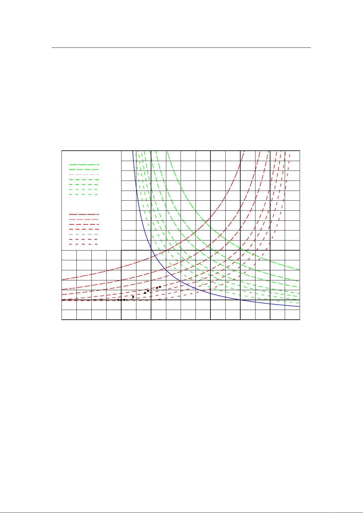
20. A Little Sky Guide
PAUL ROBINSON, WITH ADDITIONS BY ALEXANDER WOLF
This chapter lists some astronomical objects that can be located using Stellarium. All of them can be seen
with the naked eye or binoculars. Since many astronomical objects have more than one name (often having a
“proper name”, a “common name” and various catalogue numbers), the chapter lists the name as it appears
in Stellarium — use this name when using Stellarium’s search function — and any other commonly used
names.
The Location Guide entry gives brief instructions for finding each object using nearby bright stars or
groups of stars when looking at the real sky — a little time spent learning the major constellations visible
from your latitude will pay dividends when it comes to locating fainter (and more interesting!) objects. When
trying to locate these objects in the night sky, keep in mind that Stellarium displays many stars that are too
faint to be visible without optical aid, and even bright stars can be dimmed by poor atmospheric conditions
and light pollution.
20.1 Dubhe and Merak, The Pointers
Type: Stars
Magnitude: 1.83, 2.36
Location Guide: The two “rightmost” of the seven stars that form the main shape of “The Plough” (or
“Big Dipper”, part of Ursa Major).
Northern hemisphere observers are very fortunate to have two stars that point towards Polaris, which lies
very close to the Northern Celestial Pole. Whatever the time of night or season of the year, they are always
an immediate clue to the location of Polaris, the Pole Star.
20.2 M31, Messier 31, The Andromeda Galaxy
Type: Spiral Galaxy
Magnitude: 3.4
Location Guide: Find the three bright stars that constitute the main part of the constellation of Andromeda.
From the middle of these look toward the constellation of Cassiopeia.
M31 is the most distant object visible to the naked eye, and among the few nebulae that can be seen
without a telescope or powerful binoculars. Under good conditions it appears as a large fuzzy patch of light.
It is a galaxy containing billions of stars whose distance is roughly 2.5 million light years from Earth.
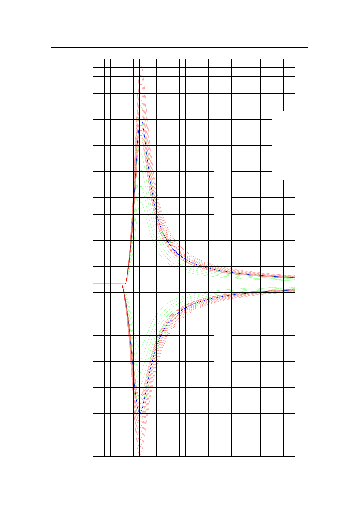
296 Chapter 20. A Little Sky Guide
20.3 The Garnet Star, µ Cephei
Type: Variable Star
Magnitude: 4.25 (Avg.)
Location Guide: Cephius lies “above” the W-shape of Cassiopeia. The Garnet Star lies slightly to one side
of a point halfway between 5 Cephei and 21 Cephei.
A “supergiant” (1035 solar radii) of spectral class M with a strong red colour. Given its name by Sir
William Herschel in the 18th century, the colour is striking in comparison to its blue-white neighbours.
20.4 4 and 5 Lyrae, ε Lyrae
Type: Double Star
Magnitude: 4.7
Location Guide: Close to Vega (α Lyrae), one of the brightest stars in the sky.
In binoculars
ε
Lyrae is resolved into two separate stars. Remarkably, each of these is also a double star
(although this will only be seen with a telescope) and all four stars form a physical system.
20.5 M13, Hercules Cluster
Type: Globular Cluster
Magnitude: 5.8
Location Guide: Located approximately 1/3 of the way along a line from 44 (η) to 40 (ζ ) Herculis.
This cluster of hundreds of thousands of mature stars appears as a circular “cloud” using the naked eye
or binoculars (a large telescope is required to resolve individual stars). Oddly the cluster appears to contain
one young star and several areas that are almost devoid of stars.
20.6 M45, The Pleiades , The Seven Sisters
Type: Open Cluster
Magnitude: 1.2 (Avg.)
Location Guide: Lies on the Bull’s back, about 1/3 between Aldebaran in Taurus and Almaak in Andromeda.
Depending upon conditions, 6 to 9 of the blueish stars in this famous cluster will be visible to someone
with average eyesight, and in binoculars it is a glorious sight. The cluster has more than 500 members in
total, many of which are shown to be surrounded by nebulous material in long exposure photographs.
20.7 C41, The Hyades
Type: Open Cluster
Magnitude: 0.5 (Avg.)
Location Guide: Lies near Aldebaran in Taurus.
The Hyades span about 6° of sky because they are one of the nearest open clusters, being about 153 light
years away. The age of the Hyades is estimated to be about 625 million years. The five brightest member
stars of the Hyades have consumed their hydrogen fuel in their cores and are now evolving into giant stars.
Four of these stars, with Bayer designations
γ
,
δ
1
,
ε
, and
θ
Tauri, form an asterism that is traditionally
identified as the head of Taurus, the Bull.
20.8 Algol, The Demon Star, β Persei
Type: Variable Star
Magnitude: 3.0 (Avg.)
Location Guide: Halfway between Aldebaran in Taurus and the middle star of the “W” of Cassiopeia.
Once every three days or so, Algol’s brightness changes from 2.1 to 3.4 and back within a matter of
hours. The reason for this change is that Algol has a dimmer giant companion star, with an orbital period of
about 2.8 days, that causes a regular partial eclipse. Although Algol’s fluctuations in magnitude have been
known since at least the 17th century, it was the first to be proved to be due to an eclipsing companion — it
is therefore the prototype Eclipsing Variable.

20.9 Sirius, α Canis Majoris 297
20.9 Sirius, α Canis Majoris
Type: Star
Magnitude: -1.47
Location Guide: Sirius is easily found by following the line of three stars in Orion’s belt southwards.
Sirius is a white dwarf star at a comparatively close 8.6 light years. This proximity and its high innate
luminance makes it the brightest star in our sky. Sirius is a double star; its companion is a white dwarf, much
dimmer but very hot, and is believed to be smaller than Earth.
20.10 M44, The Beehive, Praesepe
Type: Open Cluster
Magnitude: 3.7
Location Guide: Cancer lies about halfway between the twins (Castor & Pollux) in Gemini and Regulus,
the brightest star in Leo. The Beehive can be found between Asellus Borealis and Asellus Australis.
There are probably 350 or so stars in this cluster, although it appears to the naked eye simply as a misty
patch. It contains a mixture of stars from red giants to white dwarf and is estimated to be some 700 million
years old.
20.11 27 Cephei, δ Cephei
Type: Variable Star
Magnitude: 4.0 (Avg.)
Location Guide: Locate the four stars that form the square of Cepheus. One corner of the square has two
other bright stars nearby forming a distinctive triangle —
δ
is at the head of this triangle in the direction of
Cassiopeia.
δ
Cephei gives its name to a whole class of variables, all of which are pulsating high-mass stars in the
later stages of their evolution.
δ
Cephei is also a double star with a companion of magnitude 6.3 visible in
binoculars.
20.12 Betelgeuse, α Orionis, 58 Orionis
Type: Star
Magnitude: 0.45
Location Guide: The distinctly reddish star in the constellation of Orion – one of the shoulders of Orion.
Betelgeuse is a distinctly reddish, semiregular variable star whose apparent magnitude varies between
0.0 and 1.3. It is classified as a red supergiant of spectral type M1-2, and is one of the largest stars visible
to the naked eye. If Betelgeuse were at the center of the Solar System, its surface would extend past the
asteroid belt, completely engulfing the orbits of Mercury, Venus, Earth, Mars, and possibly Jupiter.
In 1920, Betelgeuse became the first extrasolar star to have the angular size of its photosphere measured.
Subsequent studies have reported an angular diameter (apparent size) ranging from 0.042 to 0.056 arcseconds,
with the differences ascribed to the non-sphericity, limb darkening, pulsations, and varying appearance at
different wavelengths. It is also surrounded by a complex, asymmetric envelope roughly 250 times the size
of the star, caused by mass loss from the star itself.
20.13 M42, The Great Or ion Nebula
Type: Nebula
Magnitude: 4.0
Location Guide: Almost in the middle of the area bounded by Orion’s belt and lower stars, Saiph and Rigel.
The Great Orion Nebula is the brightest nebula visible in the night sky and lies at about 1.500 light years
from Earth. It is a truly gigantic gas and dust cloud that extends for several hundred light years, reaching
almost halfway across the constellation of Orion. The nebula contains a cluster of hot young stars known as
the Trapezium, and more stars are believed to be forming within the cloud.
20.14 La Superba, Y Canum Venaticorum, HIP 62223
Type: Star
Magnitude: 5.4 (Avg.)

298 Chapter 20. A Little Sky Guide
Location Guide: Almost the center of the arch of stars of Ursa Major’s tail. Forms a neat triangle with
Phekda (γ) and Alkaid (η, tail tip) in Ursa Major towards Canes Venatici.
La Superba (215 solar radii) is a “Carbon Star” — a group of relatively cool gigantic (usually variable)
stars that have an outer shell containing high levels of carbon. This shell is very efficient at absorbing the
short wavelengths of blue light, giving carbon stars a distinctive red or orange tint. It is one of the coolest
and reddest known stars.
20.15 52 and 53 Bootis, ν
1
and
ν
2
Bootis
Type: Double Star
Magnitude: 5.0, 5.0
Location Guide: Follow a line from Seginus (
γ
Boo, left shoulder) to Nekkar (
β
Boo, the head) and then
continue for the same distance again to arrive at this double star.
This optical double star consists of a pair of different spectral types. 52 Bootis, at approximately 800
light years, is twice as far away as 53 Boo.
20.16 Almach, γ Andromedae
Type: Multiple Star
Magnitude: 2.15 (Avg.)
Location Guide: The bright star located in the “legs” of Andromeda.
In 1778, JOHANN TOBIAS MAYER discovered that
γ
Andromedae was a double star. When examined in
a small telescope, it appears to be a bright, golden-yellow star (
γ
1
Andromedae) next to a dimmer, indigo-blue
star (
γ
2
Andromedae), separated by approximately
10
′′
. It is often considered by stargazers to be a beautiful
double star with a striking contrast of color. It was later discovered that
γ
2
Andromedae is itself a triple star
system. What appears as a single star to the naked eye is thus a quadruple star system.
20.17 Algieba, γ Leonis, 41 Leonis
Type: Double Star
Magnitude: 2.20 (Avg.)
Location Guide: The third brightest star in the constellation Leo – located on the “neck” of Leo.
The bright binary system in Leo with orange-red and yellow or greenish-yellow components is visible
through a modest telescope under good atmospheric conditions. To the naked eye, the Algieba system shines
at mid-second magnitude, but a telescope easily splits the pair. On November 6, 2009, the discovery of a
planetary companion around primary star γ
1
Leonis (
γ Leonis A) was announced.
20.18 Castor, α Geminorum
Type: Multiple Star
Magnitude: 1.9 (Avg.)
Location Guide: Castor is the second-brightest object in the constellation of Gemini.
Castor is a multiple star system made up of six individual stars; there are three visual components, all of
which are spectroscopic binaries. Appearing to the naked eye as a single star, Castor was first recorded as a
double star in 1718 by JAMES POUND, but it may have been resolved into at least two sources of light by
Cassini as early as 1678. The separation between Castor A and Castor B has increased from about
2
′′
(2
arcseconds) in 1970 to about 6
′′
in 2017. These two binary pairs have magnitudes of 1.9 and 3.0.
Both components have much fainter companions, Castor Aa and Ba, and both have orbits of a few days.
Castor C, or YY Geminorum, was discovered to vary in brightness with a regular period. It is an
eclipsing binary with additional variations due to areas of different brightness on the surface of one or both
stars, as well as irregular flares. The Castor C components orbit each other in less than a day. Castor C is
believed to be in orbit around Castor AB, but with an extremely long period of several thousand years. It is
73
′′
distant from the bright components.
20.19 PZ Cas, HIP 117078
Type: Variable Star
Magnitude: 8.2 (Avg.)
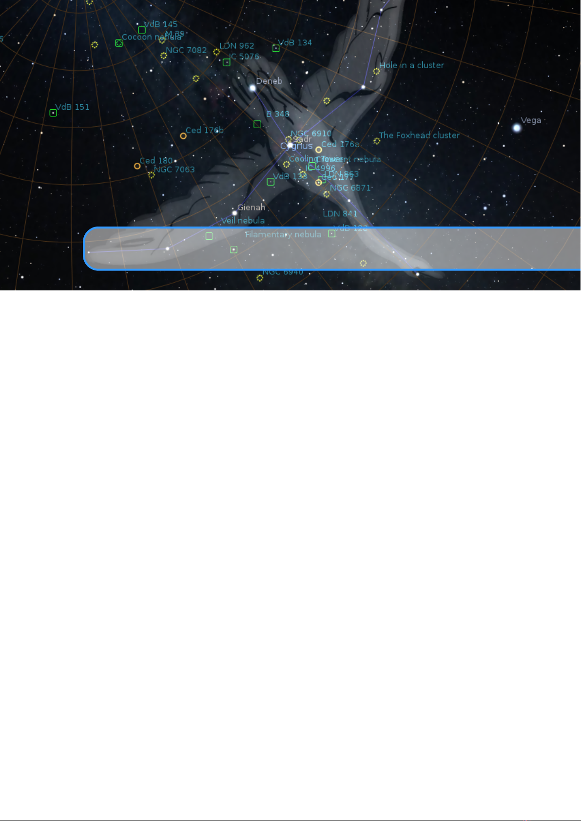
20.20 VV Cephei, HIP 108317 299
Location Guide: Lies about 1/3 between Caph (
β
Cas, the top right star of “W”) in Cassiopeia and
ι
Cephei (32 Cep, top left star in “rectangle” of Cepheus).
This faint red star is one of the biggest known stars — its average size parameter is 1565 solar radii (the
true value is from 1340 to 1940 solar radii). PZ Cas is a pulsating variable star located in a region with heavy
dust extinction.
20.20 VV Cephei, HIP 108317
Type: Variable Star, Double Star
Magnitude: 5.1 (Avg.)
Location Guide: Lies near the center of the “rectangle” of Cepheus).
This is an interesting eclipsing binary system — VV Cep A (1457 solar radii) is a highly distorted star in
a binary system, losing mass to its B-type companion VV Cephei B (10 solar radii) for at least part of its
orbit.
20.21 AH Scorpii, HIP 84071
Type: Variable Star
Magnitude: 7.1 (Avg.)
Location Guide: Lies in Scorpius, about 1
1
4
of a continuation of the Scorpion’s “tail”.
AH Sco (1411 solar radii) is variable by nearly 3 magnitudes in the visual range, and an estimated 20%
in total luminosity. The variation in diameter is not clear because the temperature also varies.
20.22 Albireo, β Cygni
Type: Double Star
Magnitude: 3.4, 5.1
Location Guide: The “head” of Cygni.
When viewed with the naked eye, it appears to be a single star. However, in a telescope it readily resolves
into a double star, consisting of Albireo A (amber), and Albireo B (blue-green). Separated by
35
′′
, the two
components provide one of the best contrasting double stars in the sky due to their different colors.
Figure 20.1: Albireo: A Bright and Beautiful Double. Credit & Copyright: Richard Yandrick.
20.23 31 and 32 Cygni, o
1
and o
2
Cygni
Type: Multiple Star
Magnitude: 3.8, 4.0
Location Guide: The two bright stars about 1/2 between Deneb (
α
Cygni, “tail” of Cygnus) and Rukh (
δ
Cygni, middle of the left “wing” of Cygnus).

300 Chapter 20. A Little Sky Guide
The wide binary
o
1
Cygni and
o
2
Cygni is separated 61
′
(NNE), and this star is an easy naked-eye
double.
o
1
Cygni with 30 Cyg and HD 192579 (HIP 99676) is a moderately difficult triple system. And
surprise — each of o
1
Cyg and o
2
Cyg are also Algol-type eclipsing binaries!
20.24 The Coathanger, Brocchi’s Cluster, Cr 399
Type: Asterism
Location Guide: It is best found by slowly sweeping across the Milky Way along an imaginary line from the
bright star Altair toward the even brighter star Vega (around 1/3 between Altair and Vega).
The asterism is made up of 10 stars ranging from 5th to 7th magnitude which form the conspicuous
“coathanger”, a straight line of 6 stars with a “hook” of 4 stars on the south side. Under a dark sky, Collinder
399 can be seen with the naked eye as an unresolved patch of light; binoculars or a telescope at very low
power are usually needed in order to view the “coathanger” asterism.
20.25 Kemble’s Cascade
Type: Asterism
Location Guide: The asterism lies in the constellation Camelopardalis, about 1/3 between CS Cam and
α
Cam — HIP 18505 has magnitude 5 and can be found in the center of the chain.
Kemble’s Cascade is a chain of stars which are visible in binoculars, even in light-polluted skies.
20.26 The Double Cluster, χ and h Persei, NGC 884 and NGC 869
Type: Open Clusters
Location Guide: The two open clusters near stars
χ and h in the constellation Perseus.
The Double Cluster (also known as Caldwell 14 or C14) is the common name for the naked-eye open
clusters NGC 869 and NGC 884 (often designated h Persei and
χ
Persei, respectively). The Double Cluster
is approximately the radiant of the Perseid meteor shower, which peaks annually around August 12 or 13.
Although easy to locate in the northern sky, observing the Double Cluster in its two parts requires optical aid.
They are described as being an “awe-inspiring” and “breathtaking” sight, and are often cited as targets in
astronomical observers’ guides.
20.27 Large Magellanic Cloud, PGC 17223
Type: Dwarf Spiral Galaxy
Magnitude: 0.9
Location Guide: It is visible as a faint “cloud” in the night sky of the southern hemisphere straddling the
border between the constellations of Dorado and Mensa, and it appears from Earth more than 20 times the
width of the full moon.
The Large Magellanic Cloud (LMC) is a satellite galaxy of the Milky Way. The Large Magellanic Cloud
is usually considered an irregular galaxy. However, it shows signs of a bar structure, and has more recently
been reclassified as a Magellanic-type dwarf spiral galaxy. At a distance of 50 kiloparsecs, the LMC is
the third closest galaxy to the Milky Way, after the Sagittarius Dwarf Spheroidal (~16 kiloparsecs) and the
putative Canis Major Dwarf Galaxy (~12.9 kiloparsecs, though its status as a galaxy is under dispute) lying
closer to the center of the Milky Way. The LMC has a diameter of about 14,000 light-years (~4.3 kpc) and a
mass of approximately 10 billion (
10
10
) solar masses, making it roughly 1/100 as massive as the Milky Way.
The LMC has a wide range of galactic objects and phenomena — surveys of the galaxy have found roughly
60 globular clusters, 400 planetary nebulae, and 700 open clusters, along with hundreds of thousands of
giant and supergiant stars.
20.28 Tarantula Nebula, C 103, NGC 2070
Type: Nebula
Magnitude: 7.3
Location Guide: Part of Large Magellanic Cloud.
The Tarantula Nebula (also known as 30 Doradus) is an H II region in the Large Magellanic Cloud
(LMC). 30 Doradus has at its centre the star cluster NGC 2070 which includes the compact concentration of
stars known as R136 that produces most of the energy that makes the nebula visible. The estimated mass of

20.29 Small Magellanic Cloud, NGC 292, PGC 3085 301
Figure 20.2: Small and Large Magellanic Clouds over Paranal Observatory. Credit: ESO/J.
Colosimo.
the cluster is 450,000 solar masses, suggesting it will likely become a globular cluster in the future (Bosch,
E. Terlevich, and R. Terlevich, 2009). The closest supernova observed since the invention of the telescope,
Supernova 1987A, occurred in the outskirts of the Tarantula Nebula.
20.29 Small Magellanic Cloud, NGC 292, PGC 3085
Type: Dwarf Irregular Galaxy
Magnitude: 2.2
Location Guide: It is located mostly in the constellation of Tucana and appears as a hazy, light patch in the
night sky about 3° across, looking like a detached piece of the Milky Way. Since it has a very low surface
brightness, it is best viewed from a dark site away from city lights.
The Small Magellanic Cloud (SMC) is a dwarf galaxy near the Milky Way. It is classified as a dwarf
irregular galaxy. It has a diameter of about 7,000 light-years and has a total mass of approximately 7 billion
times the mass of the Sun. The SMC contains a central bar structure and it is speculated that it was once a
barred spiral galaxy that was disrupted by the Milky Way to become somewhat irregular. At a distance of
about 200,000 light-years, it is one of the Milky Way’s nearest neighbors. It is also one of the most distant
objects that can be seen with the naked eye.
20.30 ω Centauri cluster, C 80, NGC 5139
Type: Globular Cluster
Magnitude: 5.3
Location Guide: It is located around 1/3 between
ζ and γ Centauri.
Omega Centauri (
ω
Cen), or NGC 5139, is a globular cluster in the constellation of Centaurus that was
first identified as a non-stellar object by Edmond Halley in 1677. Located at a distance of 15,800 light-years
(4,850 pc), it is the largest globular cluster in the Milky Way at a diameter of roughly 150 light-years. It is
estimated to contain approximately 10 million stars and a total mass equivalent to 4 million solar masses.
Omega Centauri is so distinctive from the other galactic globular clusters that it is thought to have an alternate
origin as the core remnant of a disrupted dwarf galaxy (Noyola, Gebhardt, and Bergmann, 2008).

302 Chapter 20. A Little Sky Guide
20.31 47 Tucanae, C 106, NGC 104
Type: Globular Cluster
Magnitude: 4.1
Location Guide: It can be seen with the naked eye near Small Magellanic Cloud.
It is the one of brightest globular cluster in the sky, and is noted for having a very bright and dense core.
It is also one of the most massive globular clusters in the Milky Way Galaxy, containing millions of stars.
The cluster appears roughly the size of the full moon in the sky under ideal conditions.
20.32 The Coalsack Nebula, C 99
Type: Dark Nebula
Location Guide: Dark region between
α and β Crux.
The Coalsack Nebula is the most prominent dark nebula in the skies, easily visible to the naked eye as a
dark patch silhouetted against the southern Milky Way. It is located at a distance of approximately 600 light
years away from Earth. The Coalsack is important in Australian Aboriginal astronomy, and forms the head
of the Emu in the sky in several Aboriginal cultures.
Figure 20.3: The Coalsack Nebula taken by the Wide Field Imager on the MPG/ESO 2.2-metre
telescope. Credit: ESO.
20.33 Mira, o Ceti, 68 Cet
Type: Variable Star
Magnitude: 2.0–10.1
Location Guide: It is located around 1/3 between
δ and θ Ceti.
Mira (
o
Ceti) is a star estimated 200–400 light years away in the constellation Cetus. Mira is a binary
star system that consists of a red giant (Mira A) undergoing mass loss and a high temperature white dwarf
companion (Mira B) that is accreting mass from the primary. Such an arrangement of stars is known as
a symbiotic system, and this is the closest such symbiotic pair to the Sun. Mira is the brightest periodic

20.34 α Persei Cluster, Cr 39, Mel 20 303
variable in the sky that is not visible to the naked eye for part of its cycle. Its distance is uncertain. Mira A is
a well-known example of a category of long-period variable stars known as Mira variables, which are named
after it.
20.34 α Persei Cluster, Cr 39, Mel 20
Type: Open Cluster
Magnitude: 1.2
Location Guide: Around the white-yellow supergiant Mirfak, also known as
α
Persei in direction to
δ
Persei.
The Alpha Persei Cluster, also known as Melotte 20 or Collinder 39, is an open cluster in the constellation
of Perseus. To the naked eye, the cluster consists of several blue (spectral class B) stars.
20.35 M7, The Ptolemy Cluster
Type: Open Cluster
Magnitude: 3.3
Location Guide: The cluster is easily detectable with the naked eye, close to the “sting” of Scorpius — near
the center of the line between Shaula (λ Scorpii) and Kaus Media (δ Sagittarii).
M7 has been known since antiquity — it was first recorded by the 2nd-century Greek-Roman astronomer
Ptolemy, who described it as a nebula in 130 AD. Telescopic observations of the cluster reveal about 80 stars
within a field of view of 1.3 ° across. At the cluster’s estimated distance of 980 light years this corresponds to
an actual diameter of 25 light years.
20.36 M22, NGC 6656, The Great Sagittarius Cluster
Type: Globular Cluster
Magnitude: 5.1
Location Guide: Located just south of the Ecliptic, and northwest of
λ
Sagittarii (Kaus Borealis), the
northernmost star of the “Teapot” asterism.
M22 is an elliptical globular cluster of stars in the constellation Sagittarius, near the Galactic bulge
region. It is one of the brightest and nearest globular clusters that is visible in the night sky. M22 is very
unusual in that it is one of only four globulars that are known to contain a planetary nebula. In 2012 two
black holes of between 10 and 20 solar masses each have been discovered in this globular cluster, initially
with the Very Large Array radio telescope in New Mexico, and corroborated by the Chandra X-ray telescope.
The angular size of M22 is over 0.5°.
20.37 M24, The Sagittarius Star Cloud
Type: Star Cloud
Magnitude: 4.6
Location Guide: In the Milky Way region near Polis (
µ Sagittarii).
The Sagittarius Star Cloud is a star cloud in the constellation of Sagittarius, approximately 600 light years
wide. The stars, clusters and other objects comprising M24 are part of the Sagittarius or Sagittarius-Carina
arms of the Milky Way galaxy. Messier described M24 as a “large nebulosity containing many stars” and
gave its dimensions as being some 1.5° across.
20.38 IC 4665, The Summer Beehive Cluster
Type: Open Cluster
Magnitude: 4.2
Location Guide: Visible to the naked eye near Cebalrai (
β Ophiuchi).
IC 4665 is an open cluster in the constellation Ophiuchus which is easily visible in the smallest of
telescopes and also with binoculars. From a sufficiently dark place it is also visible to the naked eye.

304 Chapter 20. A Little Sky Guide
20.39 The E Nebula, Bar nard 142 and 143
Type: Dark Nebula
Location Guide: A well-defined dark area on a background of Milky Way near Tarazed (
γ Aquilae).
The “E” or “Barnard’s E” Nebula (officially designated as B142 and B143) is a pair of dark nebulae in
the constellation Aquila. It is a well-defined dark area on a background of the Milky Way. The size of the
nebula is roughly 0.5°, and its distance from Earth is estimated at about 2000 light years.
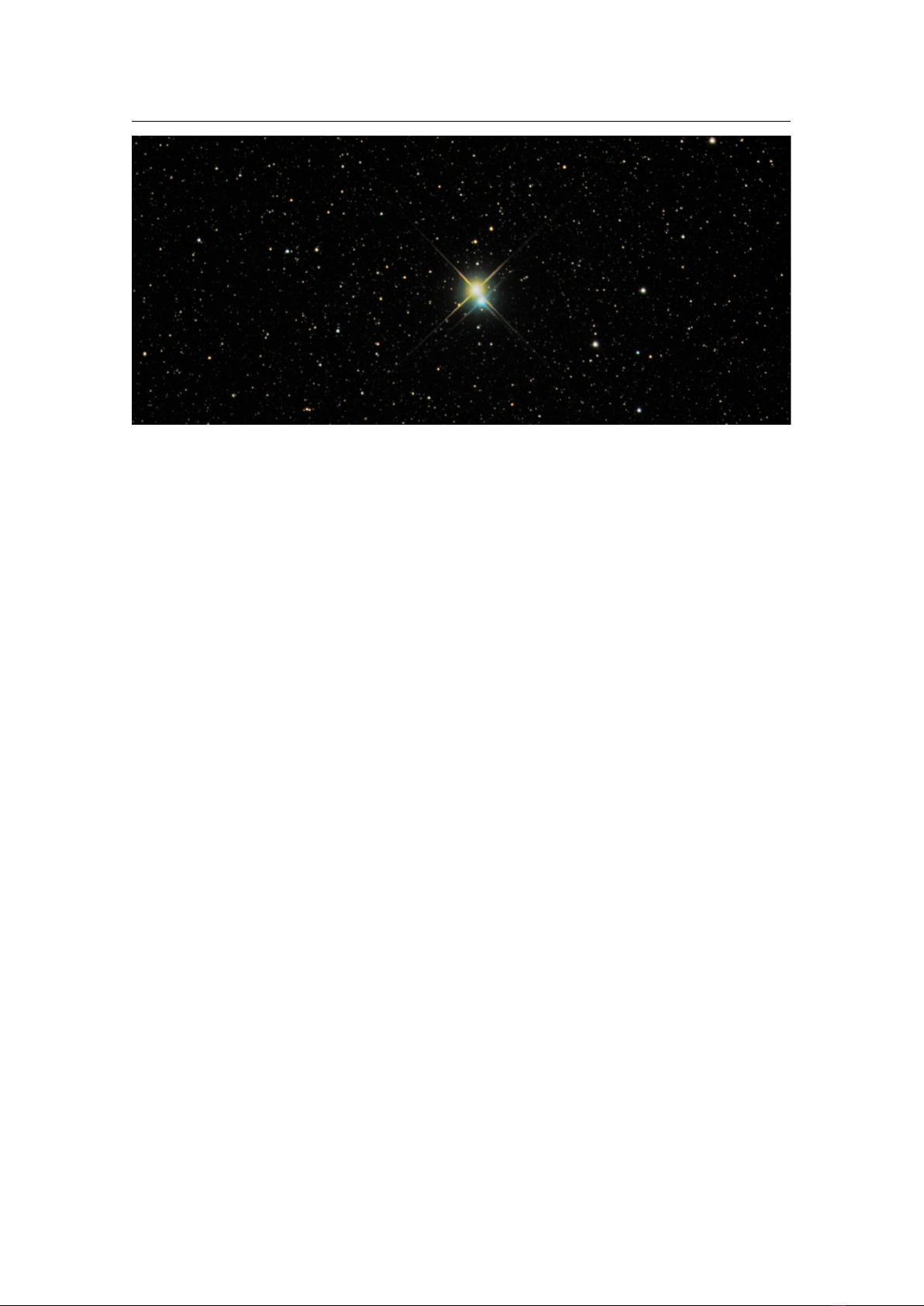
21. Exercises
PAUL ROBINSON, WITH ADDITIONS BY ALEXANDER WOLF
21.1 Find M31 in Binoculars
M31 – the Andromeda Galaxy – is the most distant object visible to the naked eye. Finding it in binoculars is
a rewarding experience for new-comers to observing.
21.1.1 Simulation
1.
Set the location to a mid-Northern latitude if necessary (M31 isn’t always visible for Southern
hemisphere observers). The UK is ideal.
2.
Find M31 and set the time so that the sky is dark enough to see it. The best time of year for this at
Northern latitudes is Autumn/Winter, although there should be a chance to see it at some time of night
throughout the year.
3.
Set the field of view to
6
° (or the field of view of your binoculars if they’re different.
6
° is typical for
7x50 binoculars).
4.
Practice finding M31 from the bright stars in Cassiopeia and the constellation of Andromeda. Learn
the chain of stars that extends from Andromeda’s central star perpendicular to her body.
21.1.2 For Real
This part is not going to be possible for many people. First, you need a good night and a dark sky. In urban
areas with a lot of light pollution it’s going to be very hard to see Andromeda.
21.2 Handy Angles
As described in section 18.5.2, your hand at arm’s length provides a few useful estimates for angular size.
It’s useful to know whether your handy angles are typical, and if not, what they are. The method here below
is just one way to do it – feel free to use another method of your own construction!
Hold your hand at arm’s length with your hand open – the tips of your thumb and little finger as far apart
as you can comfortably hold them. Get a friend to measure the distance between your thumb and your eye,
we’ll call this
D
. There is a tendency to over-stretch the arm when someone is measuring it – try to keep the
thumb-eye distance as it would be if you were looking at some distant object.
Without changing the shape of your hand, measure the distance between the tips of your thumb and little
finger. It’s probably easiest to mark their positions on a piece of paper and measure the distance between
the marks, we’ll call this
d
. Using some simple trigonometry, we can estimate the angular distance
θ
using
equation (18.5).
Repeat the process for the distance across a closed fist, three fingers and the tip of the little finger.
For example, for one author D = 72cm, d = 21cm, so:
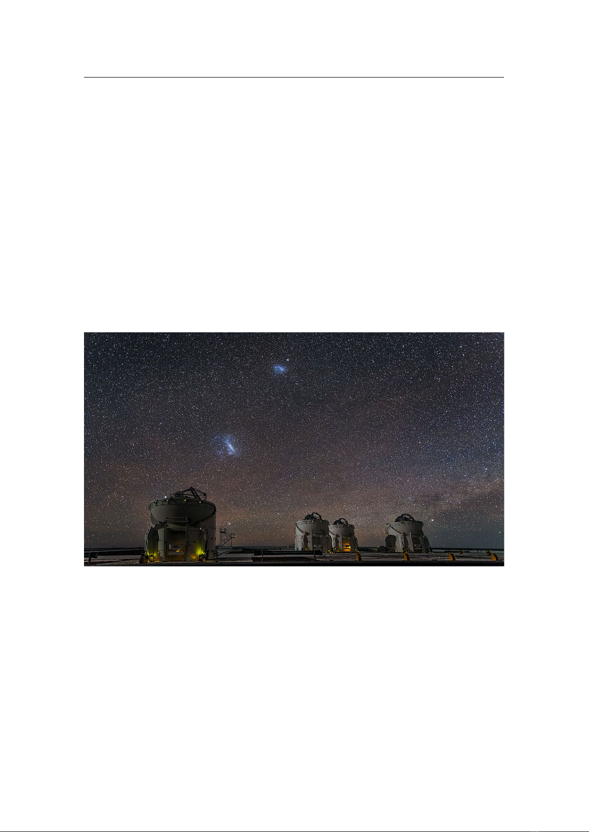
306 Chapter 21. Exercises
θ = 2 ⋅ arctan
21
144
≈ 16
1
2
° (21.1)
Remember that handy angles are not very precise – depending on your posture at a given time the values
may vary by a fair bit.
21.3 Find a Lunar Eclipse
Stellarium comes with two scripts for finding lunar eclipses, but can you find one on a different date?
21.4 Find a Solar Eclipse
Find a Solar Eclipse using Stellarium and take a screenshot of it. Use the location panel and see how the
eclipse look on different locations at the same time. Don’t forget to have “Topocentric coordinates” enabled
in the settings (see section 18.9.1).
21.5 Find a retrograde motion of Mars
Find Mars using Stellarium and take a series of screenshots of its position at different times. Use the date
and time panel and see how the motion of Mars changes over the time. Find periods of direct and retrograde
motion of Mars (see also section 17.6).
21.6 Analemma
Set a time around noon and set time rate to pause, turn on the azimuthal grid. Find the Sun and check its
horizontal coordinates. Use the date and time panel and see how the horizontal coordinates of the Sun
change over time (please use one time step for simulation — look at the position of the Sun every 7 days for
example). Use the location panel and see how the positions of the Sun look from different location at the
same times. Check the change of positions of the Sun on Mars at the same times.
21.7 Transit of Venus
Set date to
6
th
of June, 2012, find Venus near the Sun and change scale of the view (zoom in). Find time of
all four contacts and maximum of transit for your location. Because the Sun appears to rotate as it crosses
the sky, Venus will appear to move on some curve — for example it will be an inverted “U” shape for eastern
states of Australia. Check difference of path shape of Venus for equatorial and azimuthal mounts. Find a
few dates and times for transit of Venus in past and in future. Notice how they usually come in pairs 8 years
apart, with gaps of over 100 years between pairs.
21.8 Transit of Mercury
Set date to
9
th
of May, 2016, find Mercury near the Sun and change scale of the view (zoom in). Find time
of all four contacts and maximum of transit for your location. Because the Sun appears to rotate as it crosses
the sky, Mercury will appear to move on some curve — for example it will be an inverted “U” shape for
observers from Europe. Check difference of path shape of Mercury for equatorial and azimuthal mounts.
Find few dates and times for transit of Mercury in past and in future.
21.9 Triple shadows on Jupiter
Set date to
24
th
of January, 2015, find Jupiter and change scale of the view (zoom in). Find the time when
three shadows will be visible on the disk of Jupiter. Which moons cast those shadows? Check which moons
cause triple shadows on Jupiter at 3 June 2014. Details for this phenomenon you can find in the book
Mathematical Astronomy Morsels (Meeus, 1997).

21.10 Jupiter without satellites 307
21.10 Jupiter without satellites
Set date to
9
th
November, 2019, find Jupiter and change scale of the view (zoom in). Find time limits for the
disappearance of the moons. Which moons are on the back of the planet, and which — in front of it? Please
give answer on the same questions for 3 September 2009. Details for this phenomenon you can find in the
book Mathematical Astronomy Morsels (Meeus, 1997)
21.11 Mutual occultations of planets
Set date to
13
th
October, 1590, find Venus and change scale of the view (zoom in). Find time of minimal
separation of Venus and Mars on this date. Set typical scale of view for visual observation and check Venus
and Mars again. What would the typical observer of that time had said? Find the minimal separation between
Venus and Saturn near end of August 1771. What would the typical observer on Earth had said? Find the
minimal separation between Mars and Mercury in first half of August 2079.
Find mutual occultation of Earth and Mercury as seen from Mars near the end of November 2022. Find
mutual occultation of Saturn and Mercury as seen from Venus near the middle of May 1967.
Details for this phenomenon you can find in the books More Mathematical Astronomy Morsels (Meeus,
2002) and Mathematical Astronomy Morsels III (Meeus, 2004)
21.12 The proper motion of stars
Turn off ground and atmosphere, set time rate on pause, find the star HIP 87937 and change the scale of
the view to better see Barnard’s Star. Use the date and time panel and see how the location of the star is
changing in time (please try use one time step for simulation — look at the position of the star every year for
example). When will Barnard’s star cross the border of constellation? When has Barnard’s star crossed the
border of constellation in the past?
Please check the proper motions of Sirius (HIP 32349), Procyon (HIP 37279), 61 Cyg (HIP 104214)
and
τ
Cet (HIP 8102). Which star has the fastest proper motion? Which star has the slowest rate of proper
motion?
When will observers see Arcturus and HIP 68706 as close optical binary? Find the minimal angular
separation between θ and ε Ind in the past.
How will the appearance of following constellations change over a wide range of time (
−100000..100000
years for example): Ursa Major, Orion, Bootes?
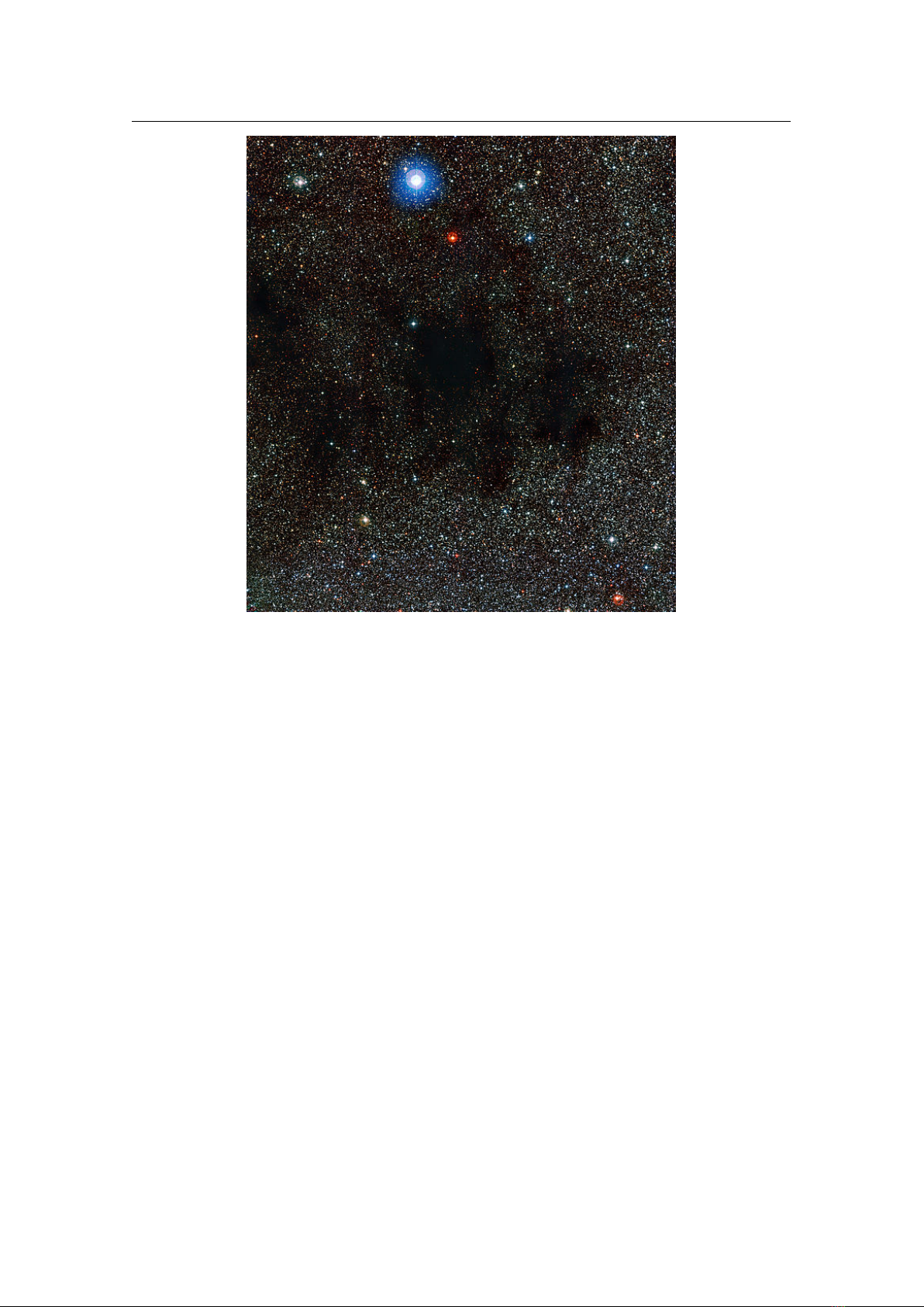

V
Appendices
A Default Hotkeys . . . . . . . . . . . . . . . . . . . . 311
B The Bortle Scale of Light Pollution
. . . . 319
C Star Catalogues
. . . . . . . . . . . . . . . . . . . . 323
D Configuration Files
. . . . . . . . . . . . . . . . . . 351
E Planetary nomenclature
. . . . . . . . . . . . 385
F Accuracy
. . . . . . . . . . . . . . . . . . . . . . . . . . 395
G GNU Free Documentation License
. . . 405
H Acknowledgements
. . . . . . . . . . . . . . . . 411
Bibliography . . . . . . . . . . . . . . . . . . . . . . . 427
Index
. . . . . . . . . . . . . . . . . . . . . . . . . . . . . . 437

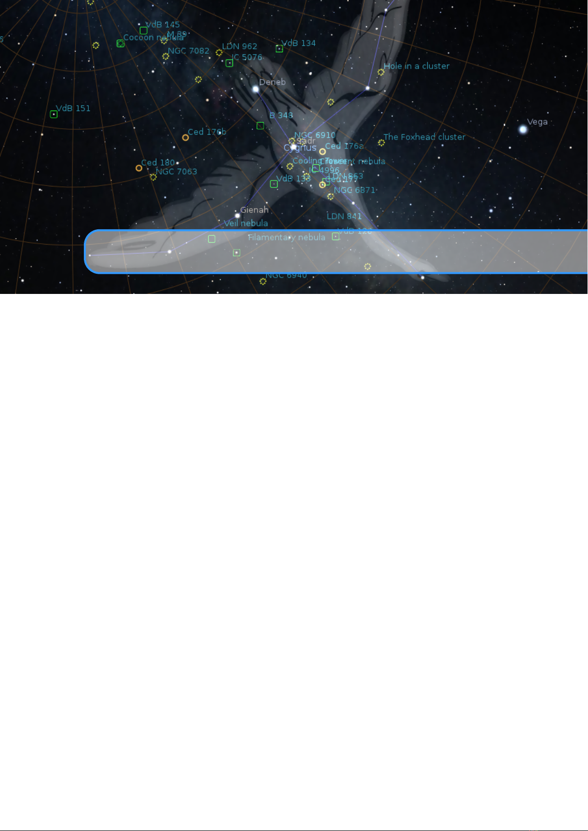
A. Default Hotkeys
The currently configured hotkeys are visible in the Help dialog (
F1
). Here is the default list for reference.
WARNING: The list of hotkeys in this Guide uses notation for standard PC-compatible keyboards. Not
all keyboards are PC-compatible – for example Apple’s computers use keyboards with their own specific keys
–
Option
and
Command
. The
Option
key is equivalent to the
Alt
key on the PC-compatible keyboards.
The Haiku operating system is the successor of BeOS, and it swaps behaviour for
Ctrl
and
Alt
keys – e.g.
PC’s
Ctrl
+
A
will be
Alt
+
A
in Haiku.
A.1 Mouse actions with combination of the keyboard keys
Actions Description
Arrow keys & left mouse drag Pan view around the sky
Page Up/Down
&
Ctrl
+
Page Up/Down
Zoom in/out
Ctrl
& left mouse drag Time dragging
Ctrl
& mouse wheel Time scrolling: minutes
Ctrl
+
& mouse wheel Time scrolling: hours
Ctrl
+
Alt
& mouse wheel Time scrolling: days
Ctrl
+
Alt
+
& mouse wheel Time scrolling: years
Left click Select object
Right click Clear selection
& left click Add custom marker
& right click Delete the one closest marker to mouse cursor
Alt
+
& right click Delete all custom markers

312 Appendix A. Default Hotkeys
A.2 Display Options
Shortcut key Description
P
Planets
Alt
+
P
Planet labels
Ctrl
+
P
Planet markers
O
Planet orbits
+
T
Planet trails
Ctrl
+
+
P
Planet selection marker
Alt
+
N
Nomenclature labels
S
Stars
Alt
+
S
Star labels
D
Deep-sky objects (symbols)
I
Deep-sky objects background images
Ctrl
+
I
Reload the deep-sky objects background images
Ctrl
+
Alt
+
D
Toggle Hierarchical Progressive Surveys (experimental)
M
Milky Way
Ctrl
+
+
Z
Zodiacal Light
G
Ground
F
Fog
+
G
Landscape Illumination
Ctrl
+
+
G
Landscape Labels
A
Atmosphere
Q
Cardinal points
,
Ecliptic line
.
Equator line
E
Equatorial grid
Z
Azimuthal grid
H
Horizon line
;
Meridian line
C
Constellation lines
V
Constellation labels
R
Constellation art
B
Constellation boundaries
Ctrl
+
Alt
+
+
V
Select single constellation
Tab
Remove selection of constellations
Ctrl
+
+
N
Native planet names (from sky culture)
Alt
+
V
Asterism labels
Alt
+
A
Asterism lines
Alt
+
R
Ray helpers
Ctrl
+
Alt
+
I
Reload the sky culture
W
Remove selection of constellations
Alt
+
W
Select all constellations
F11
Full-screen mode
Ctrl
+
N
Night mode
Ctrl
+
+
H
Flip scene horizontally
Ctrl
+
+
V
Flip scene vertically

A.3 Miscellaneous 313
A.3 Miscellaneous
Shortcut key Description
Ctrl
+
+
C
Copy selected object information to clipboard
Ctrl
+
Q
Quit
Ctrl
+
S
Save screenshot
Ctrl
+
M
Switch between equatorial and azimuthal mount
Ctrl
+
T
Toggle visibility of GUI
Ctrl
+
R
,
P
Reload shaders (for development)
A.4 Movement and Selection
Shortcut key Description
Center on selected object
Ctrl
+
H
Go to home
Ctrl
+
G
Set home planet to selected planet (“go there”)
+
E
Look towards East
+
N
Look towards North
+
S
Look towards South
+
W
Look towards West
+
Z
Look towards Zenith
Alt
+
+
N
Look towards North Celestial pole
Alt
+
+
S
Look towards South Celestial pole
T
Track object
/
Zoom in on selected object
\
Zoom out
Ctrl
+
Alt
+
1
Set FOV to 180°
Ctrl
+
Alt
+
2
Set FOV to 90°
Ctrl
+
Alt
+
3
Set FOV to 60°
Ctrl
+
Alt
+
4
Set FOV to 45°
Ctrl
+
Alt
+
5
Set FOV to 20°
Ctrl
+
Alt
+
6
Set FOV to 10°
Ctrl
+
Alt
+
7
Set FOV to 5°
Ctrl
+
Alt
+
8
Set FOV to 2°
Ctrl
+
Alt
+
9
Set FOV to 1°
Ctrl
+
Alt
+
0
Set FOV to 0.5°

314 Appendix A. Default Hotkeys
A.5 Date and Time
Shortcut key Description
=
Add 1 solar day
-
Subtract 1 solar day
Ctrl
+
=
Add 1 solar hour
Ctrl
+
-
Subtract 1 solar hour
Alt
+
=
Add 1 sidereal day
Alt
+
-
Subtract 1 sidereal day
]
Add 7 solar days
[
Subtract 7 solar days
Ctrl
+
Alt
+
+
]
Add 1 sidereal year
Ctrl
+
Alt
+
+
[
Subtract 1 sidereal year
J
Decrease time speed
+
J
Decrease time speed (a little)
K
Set normal time rate
L
Increase time speed
+
L
Increase time speed (a little)
7
Set time rate to zero
8
Set time to now
0
Set reverse time direction
Ctrl
+
D
,
P
Pause script execution
Ctrl
+
D
,
R
Resume script execution
Ctrl
+
D
,
S
Stop script execution
A.6 Scripts
Shortcut key Description
Ctrl
+
D
,
0
Run script “Solar System Screensaver”
Ctrl
+
D
,
1
Run script “Western Constellations Tour”
Ctrl
+
D
,
2
Run script “Sky Culture Tour”
Ctrl
+
D
,
3
Run script “Screensaver”
Ctrl
+
D
,
B
Run script “Skybox Tiles”
Ctrl
+
D
,
M
,
1
Run script “Jupiter and triple shadow phenomena”
Ctrl
+
D
,
M
,
2
Run script “Jupiter without Galilean satellites”
Ctrl
+
D
,
M
,
3
Run script “Occultations of bright stars by planets”
Ctrl
+
D
,
M
,
4
Run script “Mutual occultations of planets”
A.7 Windows
Shortcut key Description
F1
Toggle Help window
F2
Toggle Configuration window
F3
Toggle Search window
F4
Toggle Sky and viewing options window
F5
Toggle Date/time window
F6
Toggle Location window
F7
Toggle Shortcuts window
F10
Toggle Astronomical calculations window
F12
Toggle Script Console window
Alt
+
B
Toggle Bookmarks window

A.8 Plugins 315
A.8 Plugins
A.8.1 Angle Measure
Shortcut key Description
Ctrl
+
A
Toggle angle measurement
A.8.2 ArchaeoLines
Shortcut key Description
Ctrl
+
U
Toggle archaeolines
Ctrl
+
+
U
Toggle archaeolines dialog
A.8.3 Calendars
Shortcut key Description
Alt
+
K
Toggle Calendars display
Alt
+
+
K
Toggle Calendars dialog
A.8.4 Equation of Time
Shortcut key Description
Ctrl
+
Alt
+
T
Show solution for Equation of Time
A.8.5 Exoplanets
Shortcut key Description
Ctrl
+
Alt
+
E
Show exoplanets
Alt
+
E
Toggle Exoplanets configuration window
A.8.6 Meteor Showers
Shortcut key Description
Ctrl
+
+
M
Toggle meteor showers
+
M
Toggle radiant labels
Ctrl
+
Alt
+
M
Show search dialog
Ctrl
+
Alt
+
+
M
Show settings dialog
A.8.7 Oculars
Shortcut key Description
Ctrl
+
O
Ocular view
Alt
+
O
Oculars popup menu
Alt
+
C
Show crosshairs
Ctrl
+
B
Telrad sight
A.8.8 Pulsars
Shortcut key Description
Ctrl
+
Alt
+
P
Show pulsars

316 Appendix A. Default Hotkeys
A.8.9 Quasars
Shortcut key Description
Ctrl
+
Alt
+
Q
Show quasars
A.8.10 Satellites
Shortcut key Description
Ctrl
+
Z
Toggle satellite hints
Alt
+
+
Z
Toggle satellite labels
Alt
+
Z
Toggle Satellites configuration window
A.8.11 Scenery3d: 3D landscapes
Shortcut key Description
Ctrl
+
W
Toggle 3D landscape
Ctrl
+
+
W
Show settings dialog
Ctrl
+
Alt
+
W
Show viewpoint dialog
Ctrl
+
R
,
T
Toggle location text
Ctrl
+
R
,
S
Toggle shadows
Ctrl
+
R
,
L
Toggle torchlight
Ctrl
+
R
,
D
Toggle debug information
Ctrl
+
R
,
P
Reload shaders
A.8.12 Solar System Editor
Shortcut key Description
Ctrl
+
Alt
+
S
Import orbital elements in MPC format...
A.8.13 Telescope Control
Shortcut key Description
Ctrl
+
0
Move a telescope to a given set of coordinates (shows dialog)
Ctrl
+
1
Move telescope #1 to selected object
Ctrl
+
2
Move telescope #2 to selected object
Ctrl
+
3
Move telescope #3 to selected object
Ctrl
+
4
Move telescope #4 to selected object
Ctrl
+
5
Move telescope #5 to selected object
Ctrl
+
6
Move telescope #6 to selected object
Ctrl
+
7
Move telescope #7 to selected object
Ctrl
+
8
Move telescope #8 to selected object
Ctrl
+
9
Move telescope #9 to selected object
Alt
+
1
Move telescope #1 to the point currently in the center of the screen
Alt
+
2
Move telescope #2 to the point currently in the center of the screen
Alt
+
3
Move telescope #3 to the point currently in the center of the screen
Alt
+
4
Move telescope #4 to the point currently in the center of the screen
Alt
+
5
Move telescope #5 to the point currently in the center of the screen
Alt
+
6
Move telescope #6 to the point currently in the center of the screen
Alt
+
7
Move telescope #7 to the point currently in the center of the screen
Alt
+
8
Move telescope #8 to the point currently in the center of the screen
Alt
+
9
Move telescope #9 to the point currently in the center of the screen
A.9 Special local keys 317
Ctrl
+ +
0
Move a telescope to a given set of coordinates (shows dialog)
Ctrl
+
+
1
Sync telescope #1 to selected object
Ctrl
+
+
2
Sync telescope #2 to selected object
Ctrl
+
+
3
Sync telescope #3 to selected object
Ctrl
+
+
4
Sync telescope #4 to selected object
Ctrl
+ +
5
Sync telescope #5 to selected object
Ctrl
+
+
6
Sync telescope #6 to selected object
Ctrl
+
+
7
Sync telescope #7 to selected object
Ctrl
+
+
8
Sync telescope #8 to selected object
Ctrl
+
+
9
Sync telescope #9 to selected object
Ctrl
+
+
Alt
+
1
Abort last slew command of telescope #1
Ctrl
+
+
Alt
+
2
Abort last slew command of telescope #2
Ctrl
+
+
Alt
+
3
Abort last slew command of telescope #3
Ctrl
+
+
Alt
+
4
Abort last slew command of telescope #4
Ctrl
+
+
Alt
+
5
Abort last slew command of telescope #5
Ctrl
+
+
Alt
+
6
Abort last slew command of telescope #6
Ctrl
+
+
Alt
+
7
Abort last slew command of telescope #7
Ctrl
+
+
Alt
+
8
Abort last slew command of telescope #8
Ctrl
+
+
Alt
+
9
Abort last slew command of telescope #9
A.8.14 Text User Interface (TUI)
Shortcut key Description
Alt
+
T
Activate TUI
A.9 Special local keys
All these hotkeys are locally available to run when a specific window or tab is opened.
Shortcut key Description
Script console
Ctrl
+
+
O
Load script from file
Ctrl
+
+
S
Save script to file
Ctrl
+
Return
Run script
Astronomical calculations
+
F10
Update positions
+
F10
Calculate ephemeris
+
F10
Calculate transits
+
F10
Calculate phenomena
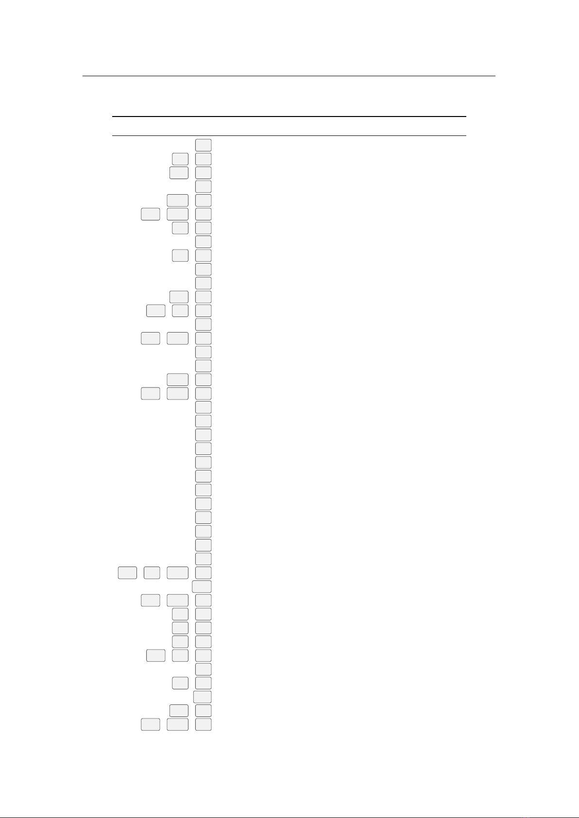
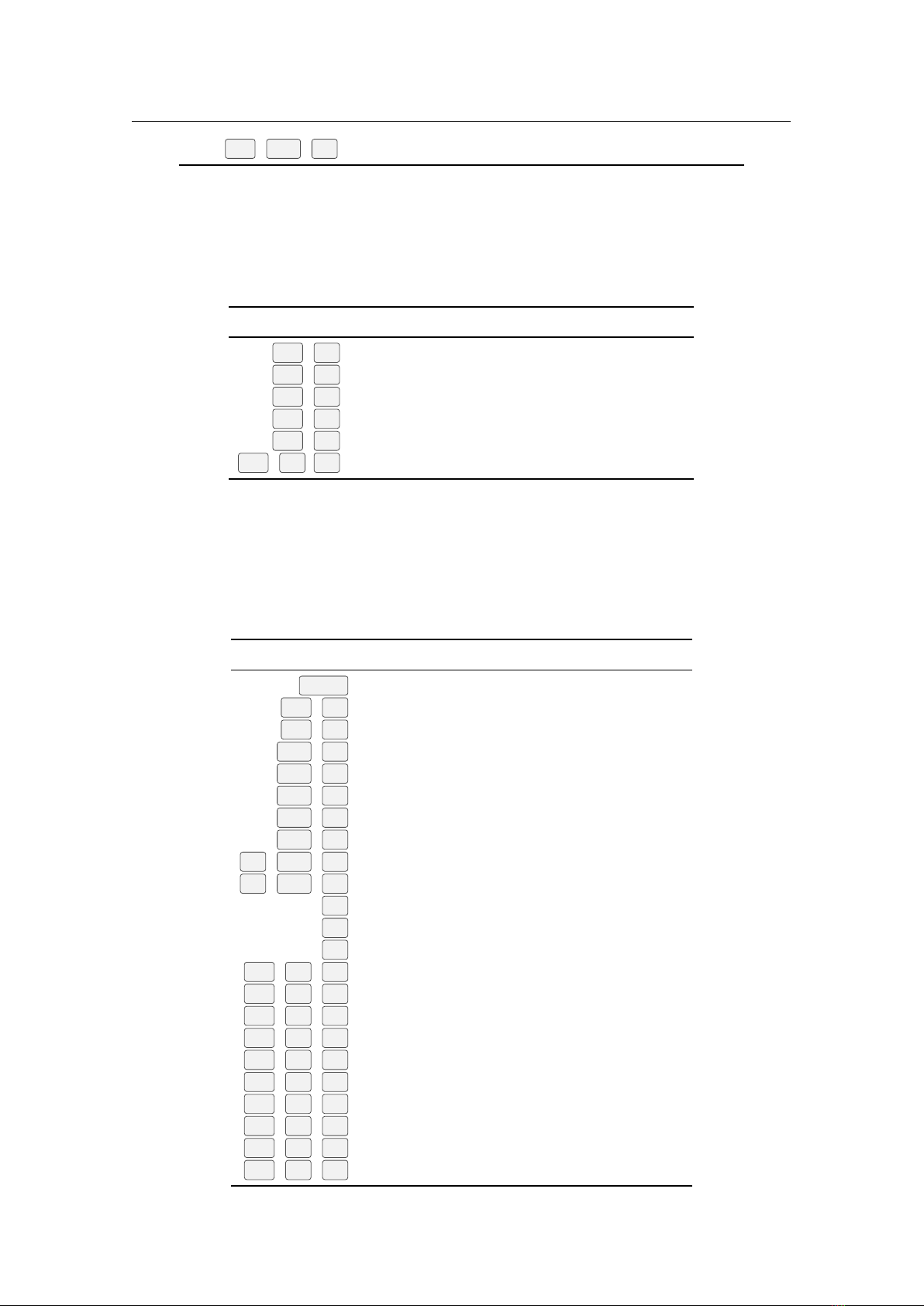
B. The Bortle Scale of Light Pollution
The Bortle scale is a nine-level numeric scale that measures the night sky’s brightness of a particular location.
It quantifies the astronomical observability of celestial objects and the interference caused by light pollution.
JOHN E. BORTLE created the scale and published it in Sky & Telescope magazine (Bortle, 2001) to help
amateur astronomers evaluate the darkness of an observing site, and secondarily, to compare the darkness
of observing sites. The scale ranges from Class 1, the darkest skies available on Earth, through Class 9,
inner-city skies. It gives several criteria for each level beyond naked-eye limiting magnitude (NELM). The
accuracy and utility of the scale have been questioned in recent research (Crumey, 2014).
Figure B.1: Light Pollution Simulation / Bortle Scale
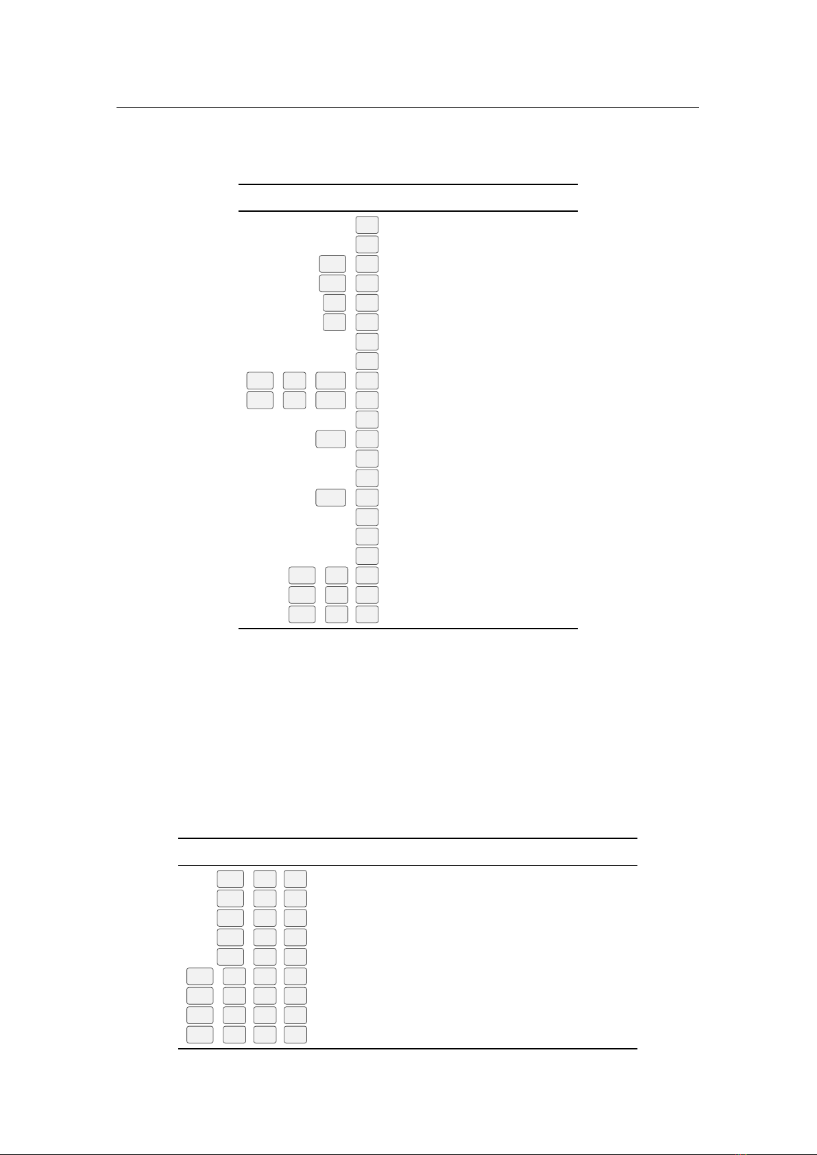
320 Appendix B. The Bortle Scale of Light Pollution
B.1 Excellent dark sky site
Level: 1
Naked-eye limiting magnitude: 7.6 – 8.0
Approx. SQM mag/arcsec
2
: 21.7 – 22.0
1
Zodiacal light, gegenschein, zodiacal band visible; M33 direct vision naked-eye object; Scorpius and
Sagittarius regions of the Milky Way cast obvious shadows on the ground; Airglow is readily visible; Jupiter
and Venus affect dark adaptation; surroundings basically invisible.
B.2 Typical truly dark site
Level: 2
Naked-eye limiting magnitude: 7.1 – 7.5
Approx. SQM mag/arcsec
2
: 21.5 – 21.7
Airglow weakly visible near horizon; M33 easily seen with naked eye; highly structured Summer Milky
Way; distinctly yellowish zodiacal light bright enough to cast shadows at dusk and dawn; clouds only visible
as dark holes; surroundings still only barely visible silhouetted against the sky; many Messier globular
clusters still distinct naked-eye objects.
B.3 Rural sky
Level: 3
Naked-eye limiting magnitude: 6.6 – 7.0
Approx. SQM mag/arcsec
2
: 21.3 – 21.5
Some light pollution evident at the horizon; clouds illuminated near horizon, dark overhead; Milky Way
still appears complex; M15, M4, M5, M22 distinct naked-eye objects; M33 easily visible with averted vision;
zodiacal light striking in spring and autumn, color still visible; nearer surroundings vaguely visible.
B.4 Rural/suburban transition
Level: 4
Naked-eye limiting magnitude: 6.1 – 6.5
Approx. SQM mag/arcsec
2
: 20.4 – 21.3
Light pollution domes visible in various directions over the horizon; zodiacal light is still visible, but
not even halfway extending to the zenith at dusk or dawn; Milky Way above the horizon still impressive,
but lacks most of the finer details; M33 a difficult averted vision object, only visible when higher than 55°;
clouds illuminated in the directions of the light sources, but still dark overhead; surroundings clearly visible,
even at a distance.
1
Dark Skies Awareness – http://www.darkskiesawareness.org/nomogram.php
B.5 Suburban sky 321
B.5 Suburban sky
Level: 5
Naked-eye limiting magnitude: 5.6 – 6.0
Approx. SQM mag/arcsec
2
: 19.1 – 20.4
Only hints of zodiacal light are seen on the best nights in autumn and spring; Milky Way is very weak or
invisible near the horizon and looks washed out overhead; light sources visible in most, if not all, directions;
clouds are noticeably brighter than the sky.
B.6 Bright suburban sky
Level: 6
Naked-eye limiting magnitude: 5.1 – 5.5
Approx. SQM mag/arcsec
2
: 18.0 – 19.1
Zodiacal light is invisible; Milky Way only visible near the zenith; sky within 35° from the horizon
glows grayish white; clouds anywhere in the sky appear fairly bright; surroundings easily visible; M33 is
impossible to see without at least binoculars, M31 is modestly apparent to the unaided eye.
B.7 Suburban/urban transition
Level: 7
Naked-eye limiting magnitude: 4.6 – 5.0
Approx. SQM mag/arcsec
2
: 18.0 – 19.1
Entire sky has a grayish-white hue; strong light sources evident in all directions; Milky Way invisible;
M31 and M44 may be glimpsed with the naked eye, but are very indistinct; clouds are brightly lit; even in
moderate-sized telescopes the brightest Messier objects are only ghosts of their true selves.
B.8 City sky
Level: 8
Naked-eye limiting magnitude: 4.1 – 4.5
Approx. SQM mag/arcsec
2
: <18.0
Sky glows white or orange — you can easily read; M31 and M44 are barely glimpsed by an experienced
observer on good nights; even with telescope, only bright Messier objects can be detected; stars forming
familiar constellation patterns may be weak or completely invisible.
B.9 Inner-city sky
Level: 9
Naked-eye limiting magnitude: 4.0 at best
Approx. SQM mag/arcsec
2
: <18.0
Sky is brilliantly lit with many stars forming constellations invisible and many weaker constellations
invisible; aside from Pleiades, no Messier object is visible to the naked eye; only objects to provide fairly
pleasant views are the Moon, the Planets and a few of the brightest star clusters.
C. Star Catalogues
This chapter provides technical descriptions on how Stellarium records its star catalogues, and the related
file formats.
C.1 Stellarium’s Sky Model
C.1.1 Zones
The celestial sphere is split into zones, which correspond to the triangular faces of a geodesic sphere. The
number of zones (faces) depends on the level of sub-division of this sphere plus one global zone for high
proper motion stars that can cross zones in the past/future or stars. The lowest level, 0, is an icosahedron (20
faces + 1 global zone), subsequent levels L of sub-division give the number of zones n as:
n = 20⋅ 4
L
+ 1 (C.1)
Stellarium uses levels 0 to 8 in the existing star catalogues. So the number of zones are 21 for level 0 to
1,310,721 for level 8. Stars within the global zone are always checked if they are visible or not without any
zone restriction, since stars can move out of their original zones due to proper motion and not drawn in the
sky. Only level 0 to level 2 star catalogs have their global zone populated (i.e. level 3-8 global zones are
empty).
For level 0, any stars who will move out of their original zones in
±200, 000
years are moved to the
global zone. For level 1 and 2, stars are moved to the global zone only if they move out of their original
zones and the bordering zones or brighter than 0.3 mag from their present apparent magnitude in
±200, 000
years.
C.2 Star Catalogue File Format
With version 25.1, Stellarium is adopting the currently most modern class of astrometrical data: Gaia DR3.
v 25.1
This astrometry satellite, operated by ESA, delivers unprecedented accuracy for millions of stars. However,
just those stars most important to human casual observers, naked-eye stars, are too bright for the sensitive
instruments. Therefore, for the brightest stars, data from the preceding Hipparcos mission are still used.
Most indexing is still based on Hipparcos numbers. In previous versions, dimmer stars were stored without
number. Now, you can use the long index from Gaia DR3 in descriptions of constellations, or search for the
number directly.
Information about the previous format is easiest found in the v24.4 User Guide.
C.2.1 General Description
Stellarium’s star catalogue data is kept in the
stars/hip_gaia3
sub-directory of the Installation Directory
v 25.1

324 Appendix C. Star Catalogues
and/or User Directory (see section 5.1).
1
The main catalogue data is split into several files:
stars_0_0v0_18.cat
stars_1_0v0_15.cat
stars_2_0v0_16.cat
stars_3_0v0_10.cat
stars_4_1v0_6.cat
stars_5_1v0_6.cat
stars_6_1v0_4.cat
stars_7_1v0_4.cat
stars_8_2v0_3.cat
There also exist some control and reference files:
object_types_v0_1.cat
stars_hip_sp_0v0_6.cat
gcvs.cat
wds_hip_part.dat
cross-id.cat
starsConfig.json
name.fab
binary_orbitparam.dat
When Stellarium starts, it reads the file
stars/hip_gaia3/starsConfig.json
2
, from which it de-
termines the names of the other files which it then loads. The file
stars_hip_sp_0v0_6.cat
contain
spectral type of HIP stars. The file
object_types_v0_1.cat
contain object type classification name for
the main star catalogs. The file
gcvs.cat
contains data about variables stars (see section C.3) and file
wds_hip_part.dat
contains data about double stars (see section C.4) which again contains references into
the main catalogue files. The file
cross-id.cat
(see section C.5) contains cross-identification data between
HIP, Gaia DR3, SAO, HD and HR designations. The file
binary_orbitparam.cat
(see section C.6)
contains binary star system orbital parameters.
A given catalogue file models stars for one and only one level (i.e. for a fixed number of zones), which
is recorded in the header of the file. Individual star records do not contain full positional coordinates, instead
they contain coordinates relative to the central position of the zone they occupy. Thus, when parsing star
catalogues, it is necessary to know about the zone model to be able to extract positional data.
File Data Data Geodesic #Records Notes
Type Record Size Level
stars_0_0v0_18.cat 0 48 bytes 0 5,045 Hipparcos + Gaia
stars_1_0v0_15.cat 0 48 bytes 1 21,611 Hipparcos + Gaia
stars_2_0v0_16.cat 0 48 bytes 2 141,761 Hipparcos + Gaia
stars_3_0v0_10.cat 0 48 bytes 3 418,129 Gaia
stars_4_1v0_6.cat 1 32 bytes 4 1,741,849 Gaia
stars_5_1v0_6.cat 1 32 bytes 5 8,051,933 Gaia
stars_6_1v0_4.cat 1 32 bytes 6 29,879,734 Gaia
stars_7_1v0_4.cat 1 32 bytes 7 57,534,724 Gaia
stars_8_2v0_3.cat 2 16 bytes 8 122,908,184 Gaia
For a given catalogue file, there may be one of three formats for the actual star data. The variation comes
from the source of the data – the larger catalogues of fainter stars providing less data per star than the brighter
star catalogues. See tables Stellarium’s star catalogue and for details.
Stellarium’s star catalogues are based on Hipparcos (Anderson and Francis, 2012; ESA, 1997) and
Gaia (Gaia Collaboration and al., 2016) catalogues.
C.2.2 File Sections
The catalogue files are split into three main sections as described in table C.1.
1
The data has significantly changed in version 25.1. The previous structure can be found in older guides.
2
Or stars/hip_gaia3/defaultStarsConfig.json file in Installation Directory
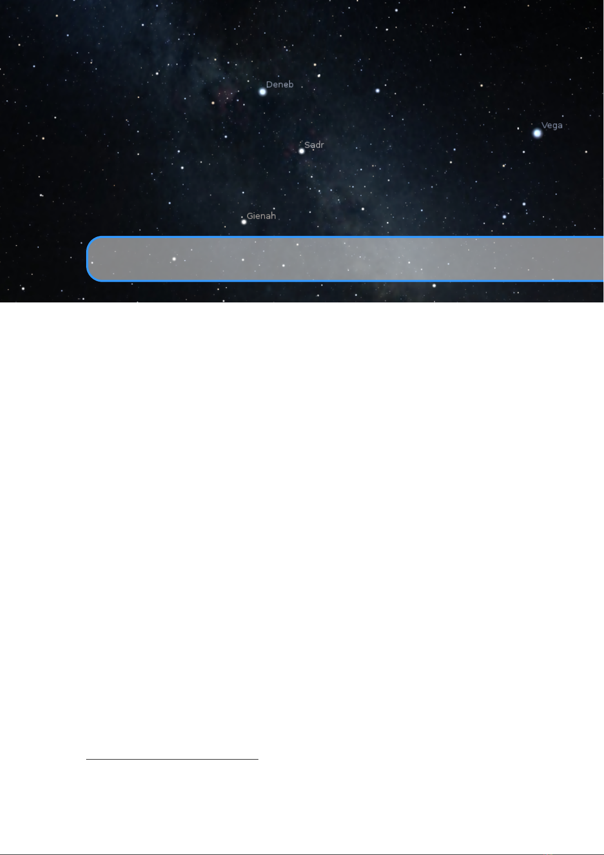
C.2 Star Catalogue File Format 325
Section Offset Description
File Header Record 0
Contains magic number, geodesic subdivision level, magnitude
and epoch information
Zone Records 28
A list of how many records there are for each zone. The length
of the zones section depends on the level value from the header
Star Data Records 28+ 4n
This section of the file contains fixed-size star records, as de-
scribed below. Records do not contain zone information, which
must be inferred by counting how many records have been read
so far and switching zones when enough have been read to fill
the number of stars for the zone, as specified in the zones sec-
tion above. The value of
n
used in the offset description is the
number of zones, as described above.
Table C.1: File sections
C.2.3 Record Types
C.2.3.1 File Header Record
The File Header Record describes file-wide settings. It also contains a magic number which servers as a file
type identifier. See table C.2.
Name Offset Type Size Description
Magic 0 int 4
magic number which identifies the file as a star
catalogue. 0x835f040a
Data Type 4 int 4
type of the file, which defines the size and struc-
ture of the Star Data record for the file.
Major Version 8 int 4 file format major version number
Minor Version 12 int 4 file format minor version number
Level 16 int 4
sets the level of sub-division of the geodesic
sphere used to create the zones. 0 means an
icosahedron (20 triangular faces + 1 global zone),
subsequent levels of sub-division lead to num-
bers of zones as described in section C.2.3.2
Magnitude Minimum 20 int 4
low bound of the magnitude of the catalog in
milli-mag unit.
Catalog Epoch 24 float 4 Epoch of the catalog in Julian days.
Table C.2: Header Record
C.2.3.2 Zone Records
The Zone Records section of the file lists the number of star records there are per zone. The number of
zones is determined from the level value in the File Header Record, as described in section C.1.1. The Zones
section is simply a list of integer values which describe the number of stars for each zone. The total length of
the Zones section depends on the number of zones. See table C.3.
C.2.3.3 Star Data Records
After the Zones section, the actual star data starts. The star data records themselves do not contain the zone
in which the star belongs. Instead, the zone is inferred from the position of the record in the file. For example,
if the Zone Records section of the file says that the first 100 records are for zone 0, the next 80 for zone 1 and
so on, it is possible to infer the zone for a given record by counting how many records have been read so far.
The actual record structure depends on the value of the Data Type, as found in the File Header Record.
See tables C.4, C.5 and C.6 for record structure details.
Details about vector algebra related to astrometric calculations can be found in (van Altena, 2013).
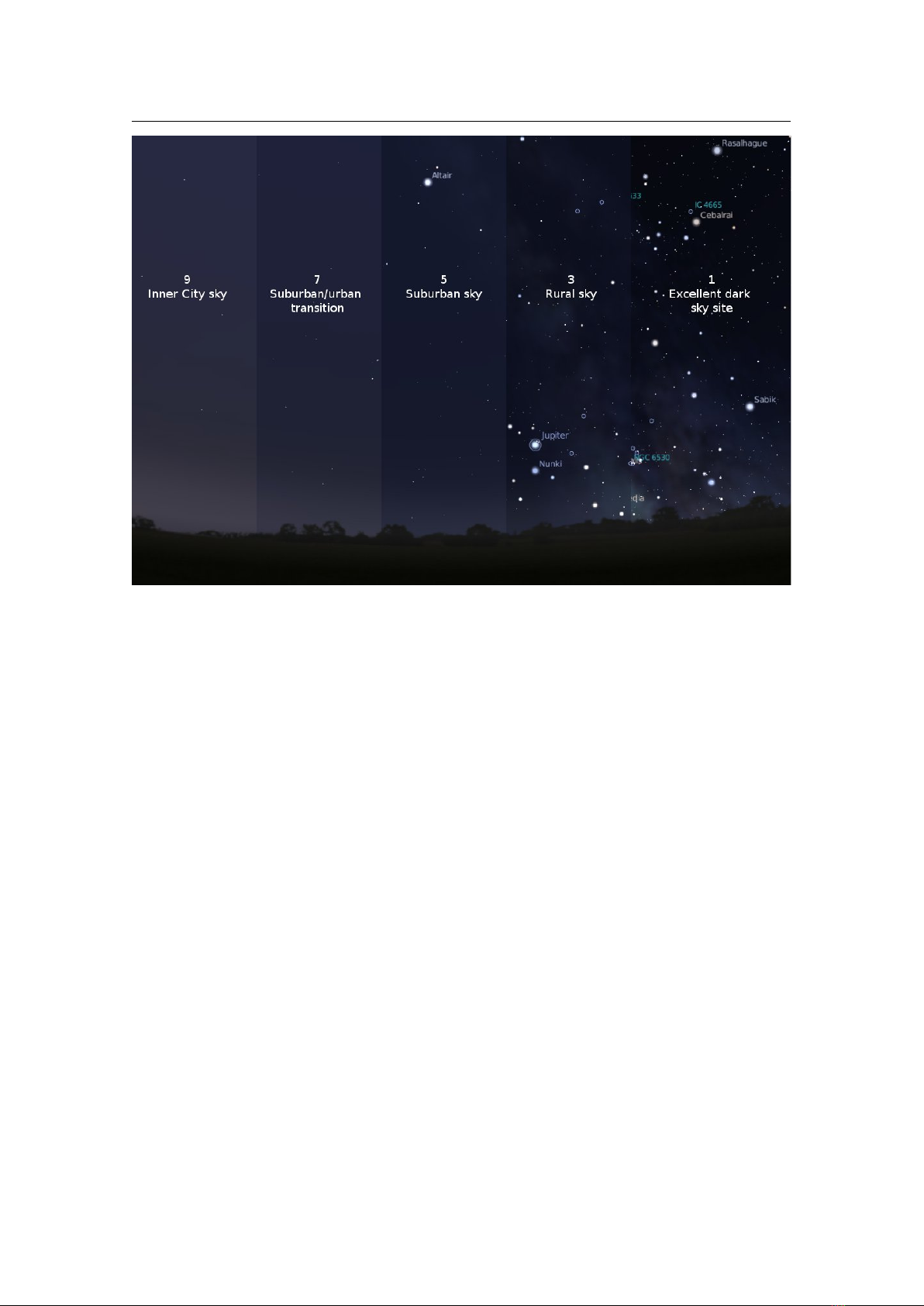
326 Appendix C. Star Catalogues
Name Offset Type Size Description
num stars in zone 0 0 int 4
number of records in this file which are in zone
0
num stars in zone 1 4 int 4
number of records is this file which are in zone
1
. . .
num stars in zone n − 1 4n − 4 int 4
number of records is this file which are in zone
n
num stars in zone n 4n int 4
number of records is this file which are in the
global zone
Table C.3: Zones section
Name Offset Type Size Description
gaia_id 0 int64_t 8 Gaia source id
x0 8 int 4
Cartesian x position of the star on an unit sphere
at the catalog epoch scaled by 2× 10
9
x1 12 int 4
Cartesian y position of the star on an unit sphere
at the catalog epoch scaled by 2× 10
9
x2 16 int 4
Cartesian z position of the star on an unit sphere
at the catalog epoch scaled by 2× 10
9
dx0 20 int 4
First component of the star’s proper motion vector
at the catalog epoch scaled by 1× 10
3
dx1 24 int 4
Second component of the star’s proper motion
vector at the catalog epoch scaled by 1× 10
3
dx2 28 int 4
Third component of the star’s proper motion vec-
tor at the catalog epoch scaled by 1× 10
3
b_v 32 short 2 B − V colour in milli-mag unit.
mag 34 short 2 V -band magnitude in milli-mag unit.
plx 36 unsigned short 2 parallax of the star in 0.02 mas unit.
plx_err 38 unsigned short 2 parallax error of the star in 0.01 mas unit.
rv 40 short 2 radial velocity of the star in 0.1 km/s unit.
sp_int 42 unsigned short 2
index into an array of spectral type descriptions
which is taken from the file
stars_hip_sp.cat
,
the index corresponds to the line number in the
file - 1
obtype 44 unsigned char 1
object type classification index. The index
corresponds to the line number in the file
object_types_v*.cat - 1.
hip 45 int 3
Hipparcos catalogue number with component ID
(e.g. A, B, C...)
Table C.4: Star Data Record Type 0

C.2 Star Catalogue File Format 327
For the catalog with Star Data Record Type 0, in practice to convert
x0, x1, x2
to right ascension
α
and
declination δ , one can use the following formulas:
α = arctan2(x1, x0)
δ = arcsin(x2)
(C.2)
and to convert proper motion vector
(dx0, dx1, dx2)
to proper motion in right ascension
µ
α
∗
and
declination µ
δ
, one can use the following formulas:
xy =
x0
2
+ x1
2
;
p = −
x1
xy
,
x0
xy
, 0.;
q = −
x0 ⋅ x2
xy
, −
x1 ⋅ x2
xy
, xy;
µ
α
∗
=
p ⋅ (dx0, dx1, dx2);
µ
δ
=
q ⋅ (dx0, dx1, dx2);
(C.3)
where
µ
α
∗
≡
µ
α
cos(δ ).
Name Offset Type Size Description
gaia_id 0 int64_t 8 Gaia source id
x0 8 int 4 Right ascension
α of the star in mas unit.
x1 12 int 4 Declination δ of the star in mas unit.
dx0 16 int 4 Proper motion
µ
α
of the star in µas/year
dx1 20 int 4 Proper motion
µ
δ
of the star in µas/year
b_v 24 short 2 B − V colour in milli-mag unit.
mag 26 short 2 V -band magnitude in milli-mag unit.
plx 28 unsigned short 2 parallax of the star in 0.01 mas unit.
plx_err 30 unsigned short 2 parallax error of the star in 0.01 mas unit.
Table C.5: Star Data Record Type 1
Name Offset Type Size Description
gaia_id 0 int64_t 8 Gaia source id
x0 8 int 3 Right ascension
α of the star in 0.1 arcsecond unit.
x1 11 int 3 Declination δ of the star in 0.1 arcsecond unit.
b_v 14 unsigned short 1 B − V colour in 25 milli-mag unit offset by +1 mag.
mag 15 unsigned short 1 V
-band magnitude in 20 milli-mag unit offset by
−16
mag.
Table C.6: Star Data Record Type 2

328 Appendix C. Star Catalogues
Name Type Description
HIP/Gaia int
This is the HIP or Gaia DR3 identifier for the star. Used for reference to
the main star catalogue.
GCVS
string This is the GCVS designation for the variable star.
Type
string Type of variability.
Max float Magnitude at maximum brightness.
MFlag
int
Magnitude flag code (0=No flag; 1="(" if max. magnitude is an amplitude;
2="<" if max. magnitude is a bright limit; 3=">" is max. magnitude is a
faint limit).
Min I
float First minimum magnitude or amplitude.
Min II float Second minimum magnitude.
V
char The photometric system for magnitudes.
Epoch
float Epoch for maximum or minimum light (in Julian days).
Period
float Period for the variable star (in days).
M-m
float Rising time or duration of the eclipse (in percent).
Spectrum
string Spectral class of the variable star.
Table C.7: Variable Star Catalog File Format
C.3 Variable Stars
Since version 0.12.2 Stellarium supports the subset of variable stars from GCVS
3
which have HIP identifiers
(i.e., stars from the Hipparcos catalog). Stellarium’s Catalog of Variable Stars is based on the “General
catalogue of variable stars: Version GCVS 5.1” (Samus’ et al., 2017).
C.3.1 Variable Star Catalog File Format
C.3.1.1 General Description
Stellarium’s Variable Stars catalog data is kept in the
stars/hip_gaia3
sub-directory of the Installation
Directory and/or User Directory (see section 5.1).
C.3.1.2 File Format
The
gcvs.cat
file contains data about 49800+ Variable Stars (see section 19.2.5) which have HIP or Gaia
DR3 identifiers and are stored in a plain text format with tab delimiter (Table C.7).
C.3.2 GCVS Variability Types
An improved system of variability classification is used in the fourth edition of the GCVS, based on recent
developments in classification principles and taking into account the suggestions of a number of specialists.
Variability types are grouped according to the major astrophysical reasons for variability.
All of these classes include objects of a dissimilar nature that belong to different types of light variability.
On the other hand, an object may be variable because of almost all of the possible reasons or because of any
combination of them. If a variable belongs to several types of variability, the types are joined in the data field
by a “+” sign, e.g., E+UG, UV+BY.
Despite considerable success in understanding stellar variability processes, the classification adopted in
the Catalogue is far from perfect. This is especially the case for explosive, symbiotic and novalike variables;
X-ray sources; and peculiar objects.
The new variability types (ZZO, AM, R, BE, BLBOO, EP, SRS, LPB) have been added in the Name-Lists
67-77 and in the GCVS vol.V.
You can read about latest different types of variability at SAI GCVS page
4
.
C.3.2.1 Eruptive Variable Stars
Eruptive variables are stars varying in brightness because of violent processes and flares occurring in their
chromospheres and coronae. The light changes are usually accompanied by shell events or mass outflow in
3
http://www.sai.msu.su/gcvs/gcvs/
4
http://www.sai.msu.su/gcvs/gcvs/vartype.htm
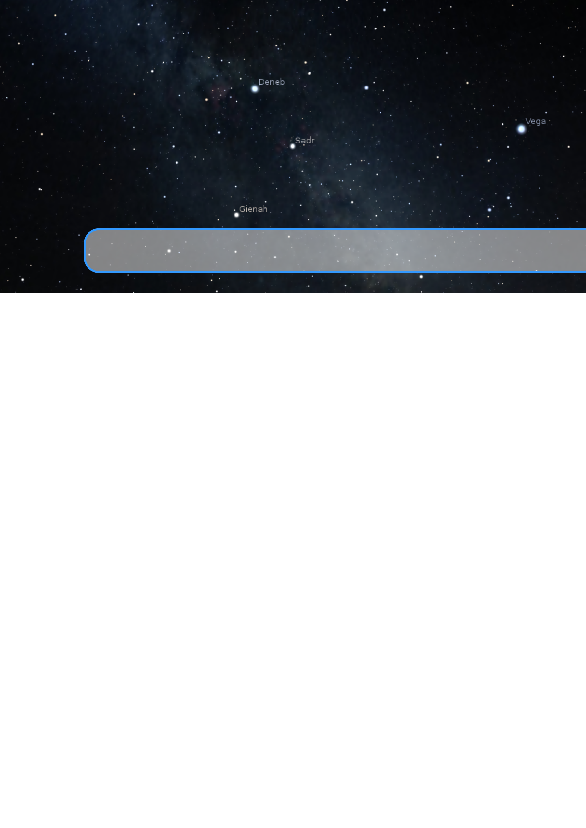
C.3 Variable Stars 329
the form of stellar winds of variable intensity and/or by interaction with the surrounding interstellar medium.
This class includes the following types:
BE
It becomes more and more clear that, although the majority of Be stars are photometrically variable,
not all of them could be properly called GCAS variables. Quite a number of them show small-scale
variations not necessarily related to shell events; in some cases the variations are quasi-periodic. By
now we are not able to present an elaborated system of classification for Be variables, but we adopt a
decision that in the cases when a Be variable cannot be readily described as a GCAS star we give
simply BE for the type of variability.
FU
Orion variables of the FU Orionis type. Characterized by gradual increases in brightness by about 6
mag in several months, followed by either almost complete constancy at maximum that is sustained
for long periods of time or slow decline by 1-2 mag. Spectral types at maximum are in the range
Ae(alpha) - Gpe(alpha). After an outburst, a gradual development of an emission spectrum is observed
and the spectral type becomes later. These variables probably mark one of the evolutionary stages of
T Tauri-type Orion variables (INT), as evidenced by an outburst of one member, V1057 Cyg, but its
decline (2.5 mag in 11 years) commenced immediately after maximum brightness was attained. All
presently known FU Ori variables are coupled with reflecting cometary nebulae.
GCAS
Eruptive irregular variables of the Gamma Cas type. These are rapidly rotating B III-IVe stars
with mass outflow from their equatorial zones. The formation of equatorial rings or disks is often
accompanied by temporary fading. Light amplitudes may reach 1.5 mag in V.
I
Poorly studied irregular variables with unknown features of light variations and spectral types. This is a
very inhomogeneous group of objects.
IA Poorly studied irregular variables of early (O-A) spectral type.
IB Poorly studied irregular variables of intermediate (F-G) to late (K-M) spectral type.
IN
Orion variables. Irregular, eruptive variables connected with bright or dark diffuse nebulae or
observed in the regions of these nebulae. Some of them may show cyclic light variations caused
by axial rotation. In the Spectrum-Luminosity diagram, they are found in the area of the main
sequence and subgiants. They are probably young objects that, during the course of further
evolution, will become light-constant stars on the zero-age main sequence (ZAMS). The range
of brightness variations may reach several magnitudes. In the case of rapid light variations
having been observed (up to 1 mag in 1-10 days), the letter “S” is added to the symbol for the
type (INS). This type may be divided into the following subtypes:
INA
Orion variables of early spectral types (B-A or Ae). They are often characterized by
occasional abrupt Algol-like fadings (T Ori);
INB
Orion variables of intermediate and late spectral types, F-M or Fe-Me (BH Cep, AH Ori).
F-type stars may show Algol-like fadings similar to those of many INA stars; K-M stars
may produce flares along with irregular light variations;
INT,IT
Orion variables of the T Tauri type. Stars are assigned to this type on the basis of
the following (purely spectroscopic) criteria: spectral types are in the range Fe-Me. The
spectra of most typical stars resemble the spectrum of the solar chromosphere. The feature
specific to the type is the presence of the fluorescent emission lines Fe II 4046, 4132 A
(anomalously intense in the spectra of these stars), emission lines [Si II] and [O I], as well
as the absorption line Li I 6707 A. These variables are usually observed only in diffuse
nebulae. If it is not apparent that the star is associated with a nebula, the letter “N” in the
symbol for the type may be omitted, e.g., IT (RW AUR);
IN(YY)
Some Orion variables (YY Ori) show the presence of absorption components on the
redward sides of emission lines, indicating the infall of matter toward the stars’ surfaces.
In such cases, the symbol for the type may be accompanied by the symbol “YY”.
IS
Rapid irregular variables having no apparent connection with diffuse nebulae and showing light
changes of about 0.5 - 1.0 mag within several hours or days. There is no strict boundary between
rapid irregular and Orion variables. If a rapid irregular star is observed in the region of a diffuse
nebula, it is considered an Orion variable and designated by the symbol INS. To attribute a
variable to the IS type, it is necessary to take much care to be certain that its light changes are
really not periodic. Quite a number of the stars assigned to this type in the third edition of the
GCVS turned out to be eclipsing binary systems, RR Lyrae variables, and even extragalactic BL
Lac objects.
ISA Rapid irregular variables of the early spectral types, B-A or Ae;
ISB Rapid irregular variables of the intermediate and late spectral types, F-M and Fe-Me.

330 Appendix C. Star Catalogues
RCB
Variables of the R Coronae Borealis type. These are hydrogen-poor, carbon- and helium-rich, high-
luminosity stars belonging to the spectral types Bpe-R, which are simultaneously eruptive and
pulsating variables. They show slow nonperiodic fadings by 1-9 mag in V lasting from a month or
more to several hundred days. These changes are superposed on cyclic pulsations with amplitudes up
to several tenths of a magnitude and periods in the range 30-100 days.
RS
Eruptive variables of the RS Canum Venaticorum type. This type is ascribed to close binary systems
with spectra showing Ca II H and K in emission, their components having enhanced chromospheric
activity that causes quasi-periodic light variability. The period of variation is close to the orbital one,
and the variability amplitude is usually as great as 0.2 mag in V (UX Ari). They are X-ray sources
and rotating variables. RS CVn itself is also an eclipsing system (see below).
SDOR
Variables of the S Doradus type. These are eruptive, high-luminosity Bpec-Fpec stars showing
irregular (sometimes cyclic) light changes with amplitudes in the range 1-7 mag in V. They belong
to the brightest blue stars of their parent galaxies. As a rule, these stars are connected with diffuse
nebulae and surrounded by expanding envelopes (P Cyg, Eta Car).
UV
Eruptive variables of the UV Ceti type, these are K Ve-M Ve stars sometimes displaying flare activity
with amplitudes from several tenths of a magnitude up to 6 mag in V. The amplitude is considerably
greater in the ultraviolet spectral region. Maximum light is attained in several seconds or dozens of
seconds after the beginning of a flare; the star returns to its normal brightness in several minutes or
dozens of minutes.
UVN
Flaring Orion variables of spectral types Ke-Me. These are phenomenologically almost identical
to UV Cet variables observed in the solar neighborhood. In addition to being related to nebulae,
they are normally characterized by being of earlier spectral type and greater luminosity, with slower
development of flares (V389 Ori). They are possibly a specific subgroup of INB variables with
irregular variations superimposed by flares.
WR
Eruptive Wolf-Rayet variables. Stars with broad emission features of He I and He II as well as C II-C
IV, O II-O IV, and N III-N V. They display irregular light changes with amplitudes up to 0.1 mag in V,
which are probably caused by physical processes, in particular, by nonstable mass outflow from their
atmospheres.
C.3.2.2 Pulsating Variable Stars
Pulsating variables are stars showing periodic expansion and contraction of their surface layers. The
pulsations may be radial or nonradial. A radially pulsating star remains spherical in shape, while in the case
of nonradial pulsations the star’s shape periodically deviates from a sphere, and even neighboring zones of
its surface may have opposite pulsation phases.
Depending on the period value, on the mass and evolutionary status of the star, and on the scale of
pulsational phenomena, the following types of pulsating variables may be distinguished:
ACYG
Variables of the Alpha Cygni type, which are nonradially pulsating supergiants of Bep-AepIa
spectral types. The light changes with amplitudes of the order of 0.1 mag often seem irregular, being
caused by the superposition of many oscillations with close periods. Cycles from several days to
several weeks are observed.
BCEP
Variables of the Beta Cephei type (Beta Cep, Beta CMa), which are pulsating O8-B6 I-V stars with
periods of light and radial-velocity variations in the range of 0.1 - 0.6 days and light amplitudes from
0.01 to 0.3 mag in V. The light curves are similar in shape to average radial-velocity curves but lag in
phase by a quarter of the period, so that maximum brightness corresponds to maximum contraction,
i.e., to minimum stellar radius. The majority of these stars probably show radial pulsations, but some
(V469 Per) display nonradial pulsations; multiperiodicity is characteristic of many of these stars.
BCEPS
A short-period group of Beta Cep variables. The spectral types are B2-B3 IV-V; periods and
light amplitudes are in the ranges 0.02 - 0.04 days and 0.015 - 0.025 days, respectively, i.e., an
order of magnitude smaller than the normally observed ones.
BLBOO
The so-called “anomalous Cepheids”, i.e. stars with periods characteristic of comparatively
long-period RRAB variables, but considerably brighter by luminosity (BL Boo = NGC 5466 V19).
CEP
Cepheids. Radially pulsating, high luminosity (classes Ib-II) variables with periods in the range of
1-135 days and amplitudes from several hundredths to 2 mag in V (in the B band, the amplitudes are
greater). Spectral type at maximum light is F; at minimum, the types are G-K. The longer the period
of light variation, the later is the spectral type. The maximum of the surface-layer expansion velocity
almost coinciding with maximum light.
CEP(B)
Cepheids (TU Cas, V 367 Sct) displaying the presence of two or more simultaneously
operating pulsation modes (usually the fundamental tone with the period P0 and the first

C.3 Variable Stars 331
overtone P1). The periods P0 are in the range from 2 to 7 days, with the ratio P1/P0 approx.
0.71.
CW
Variables of the W Virginis type. These are pulsating variables of the galactic spherical component (old
disk) population with periods of approximately 0.8 to 35 days and amplitudes from 0.3 to 1.2 mag in
V. They obey a period-luminosity relation different from that for Delta Cep variables (see DCEP). For
an equal period value, the W Vir variables are fainter than the Delta Cep stars by 0.7 - 2 mag. The
light curves of W Vir variables for some period intervals differ from those of Delta Cep variables for
corresponding periods either by amplitudes or by the presence of humps on their descending branches,
sometimes turning into broad flat maxima. W Vir variables are present in globular clusters and at high
galactic latitudes. They may be separated into the following subtypes:
CWA W Vir variables with periods longer than 8 days (W Vir);
CWB W Vir variables with periods shorter than 8 days (BL Her).
DCEP
These are the classical cepheids, or Delta Cep-type variables. Comparatively young objects that
have left the main sequence and evolved into the instability strip of the Hertzsprung-Russell (H-R)
diagram, they obey the well-known Cepheid period-luminosity relation and belong to the young disk
population. DCEP stars are present in open clusters. They display a certain relation between the
shapes of their light curves and their periods.
DCEPS
These are Delta Cep variables having light amplitudes <0.5 mag in V (<0.7 mag in B) and
almost symmetrical light curves (M-m approx. 0.4 - 0.5 periods); as a rule, their periods do not
exceed 7 days. They are probably first-overtone pulsators and/or are in the first transition across
the instability strip after leaving the main sequence (SU Cas).
Traditionally, both Delta Cep and W Vir stars are quite often called Cepheids because it is
often impossible to discriminate between them on the basis of the light curves for periods
in the range 3 - 10 days. However, these are distinct groups of entirely different objects in
different evolutionary stages. One of the significant spectral differences between W Vir stars
and Cepheids is the presence, during a certain phase interval, of hydrogen-line emission in the
former and of Ca II H and K emission in the latter.
DSCT
Variables of the Delta Scuti type. These are pulsating variables of spectral types A0-F5 III-V
displaying light amplitudes from 0.003 to 0.9 mag in V (usually several hundredths of a magnitude)
and periods from 0.01 to 0.2 days. The shapes of the light curves, periods, and amplitudes usually
vary greatly. Radial as well as nonradial pulsations are observed. The variability of some members
of this type appears sporadically and sometimes completely ceases, this being a consequence of
strong amplitude modulation with the lower value of the amplitude not exceeding 0.001 mag in some
cases. The maximum of the surface layer expansion does not lag behind the maximum light for
more than 0.1 periods. DSCT stars are representatives of the galactic disk (flat component) and are
phenomenologically close to the SX Phe variables.
DSCTC
Low amplitude group of Delta Sct variables (light amplitude <0.1 mag in V). The majority
of this type’s representatives are stars of luminosity class V; objects of this subtype generally
are representative of the Delta Sct variables in open clusters.
GDOR
Gamma Doradus stars. Early type F dwarfs showing (multiple) periods from several tenths of a day
to slightly in excess of one day. Amplitudes usually do not exceed 0.1 mag. Presumably low degree
g-mode non-radial pulsators. Prototype: gamma Dor.
L
Slow irregular variables. The light variations of these stars show no evidence of periodicity, or any
periodicity present is very poorly defined and appears only occasionally. Like for the type I, stars are
often attributed to this type because of being insufficiently studied. Many type L variables are really
semiregulars or belong to other types.
LB
Slow irregular variables of late spectral types (K, M, C, S); as a rule, they are giants (CO Cyg).
This type is also ascribed, in the GCVS, to slow red irregular variables in the case of unknown
spectral types and luminosities.
LC
Irregular variable supergiants of late spectral types having amplitudes of about 1 mag in V (TZ
Cas).
LPB The comparatively long-period pulsating B stars (periods exceeding (LBV) one day).
M
Mira (Omicron) Ceti-type variables. These are long-period variable giants with characteristic late-type
emission spectra (Me, Ce, Se) and light amplitudes from 2.5 to 11 mag in V. Their periodicity is
well pronounced, and the periods lie in the range between 80 and 1000 days. Infrared amplitudes
are usually less than in the visible and may be <2.5 mag. For example, in the K band they usually
do not exceed 0.9 mag. If the amplitudes exceed 1 - 1.5 mag , but it is not certain that the true light

332 Appendix C. Star Catalogues
amplitude exceeds 2.5 mag, the symbol “M” is followed by a colon, or the star is attributed to the
semiregular class with a colon following the symbol for that type (SR).
PVTEL
Variables of the PV Telescopii type. These are helium supergiant Bp stars with weak hydrogen
lines and enhanced lines of He and C. They pulsate with periods of approximately 0.1 to 1 days, or
vary in brightness with an amplitude of 0.1 mag in V during a time interval of about a year.
RPHS
Very rapidly pulsating hot (subdwarf B) stars. Typical periods are hundreds of seconds, amplitudes
are within several hundredths of a magnitude. Prototype: V361 Hya = EC 14026-2647.
RR
Variables of the RR Lyrae type, which are radially-pulsating giant A-F stars having amplitudes from 0.2
to 2 mag in V. Cases of variable light-curve shapes as well as variable periods are known. If these
changes are periodic, they are called the Blazhko effect.
Traditionally, RR Lyrae stars are sometimes called short-period Cepheids or cluster-type variables. The
majority of these stars belong to the spherical component of the Galaxy; they are present, sometimes
in large numbers, in some globular clusters, where they are known as pulsating horizontal-branch stars.
Like Cepheids, maximum expansion velocities of surface layers for these stars practically coincide
with maximum light.
RR(B)
RR Lyrae variables showing two simultaneously operating pulsation modes, the fundamental
tone with the period P0 and the first overtone, P1 (AQ Leo). The ratio P1/P0 is approximately
0.745;
RRAB
RR Lyrae variables with asymmetric light curves (steep ascending branches), periods from
0.3 to 1.2 days, and amplitudes from 0.5 to 2 mag in V;
RRC
RR Lyrae variables with nearly symmetric, sometimes sinusoidal, light curves, periods from
0.2 to 0.5 days, and amplitudes not greater than 0.8 mag in V (SX UMa).
RV
Variables of the RV Tauri type. These are radially pulsating supergiants having spectral types F-G at
maximum light and K-M at minimum. The light curves are characterized by the presence of double
waves with alternating primary and secondary minima that can vary in depth so that primary minima
may become secondary and vice versa. The complete light amplitude may reach 3-4 mag in V. Periods
between two adjacent primary minima (usually called formal periods) lie in the range 30-150 days
(these are the periods appearing in the Catalogue). Two subtypes, RVA and RVB, are recognized:
RVA RV Tauri variables that do not vary in mean magnitude (AC Her);
RVB
RV Tauri variables that periodically (with periods from 600 to 1500 days and amplitudes up to
2 mag in V) vary in mean magnitude (DF Cyg, RV Tau).
SR
Semiregular variables, which are giants or supergiants of intermediate and late spectral types showing
noticeable periodicity in their light changes, accompanied or sometimes interrupted by various
irregularities. Periods lie in the range from 20 to >2000 days, while the shapes of the light curves are
rather different and variable, and the amplitudes may be from several hundredths to several magnitudes
(usually 1-2 mag in V).
SRA
Semiregular late-type (M, C, S or Me, Ce, Se) giants displaying persistent periodicity and
usually small (<2.5 mag in V) light amplitudes (Z Aqr). Amplitudes and light-curve shapes
generally vary and periods are in the range of 35-1200 days. Many of these stars differ from
Miras only by showing smaller light amplitudes;
SRB
Semiregular late-type (M, C, S or Me, Ce, Se) giants with poorly defined periodicity (mean
cycles in the range of 20 to 2300 days) or with alternating intervals of periodic and slow irregular
changes, and even with light constancy intervals (RR CrB, AF Cyg). Every star of this type may
usually be assigned a certain mean period (cycle), which is the value given in the Catalogue.
In a number of cases, the simultaneous presence of two or more periods of light variation is
observed;
SRC
Semiregular late-type (M, C, S or Me, Ce, Se) supergiants (Mu Cep) with amplitudes of about
1 mag and periods of light variation from 30 days to several thousand days;
SRD
Semiregular variable giants and supergiants of F, G, or K spectral types, sometimes with
emission lines in their spectra. Amplitudes of light variation are in the range from 0.1 to 4 mag,
and the range of periods is from 30 to 1100 days (SX Her, SV UMa).
SRS
Semiregular pulsating red giants with short period (several days to a month), probably high-
overtone pulsators. Prototype: AU Ari.
SXPHE
Phenomenologically, these resemble DSCT (Delta Sct) variables and are pulsating subdwarfs of
the spherical component, or old disk galactic population, with spectral types in the range A2-F5. They
may show several simultaneous periods of oscillation, generally in the range 0.04-0.08 days, with
variable-amplitude light changes that may reach 0.7 mag in V. These stars are present in globular

C.3 Variable Stars 333
clusters.
ZZ
ZZ Ceti variables. These are nonradially pulsating white dwarfs that change their brightnesses with
periods from 30 s to 25 min and amplitudes from 0.001 to 0.2 mag in V. They usually show several
close period values. Flares of 1 mag are sometimes observed; however, these may be explained by the
presence of close UV Ceti companions.
These variables are divided into the following subtypes:
ZZA
ZZ Cet-type variables of DA spectral type (ZZ Cet) having only hydrogen absorption lines in
their spectra;
ZZB
ZZ Cet-type variables of DB spectral type having only helium absorption lines in their spectra.
ZZO
ZZ Cet-type variables of the DO spectral type showing HeII and and CIV absorption lines in
their spectra.
C.3.2.3 Rotating Variable Stars
Variable stars with nonuniform surface brightness and/or ellipsoidal shapes, whose variability is caused by
axial rotation with respect to the observer. The nonuniformity of surface brightness distributions may be
caused by the presence of spots or by some thermal or chemical inhomogeneity of the atmosphere caused
by a magnetic field whose axis is not coincident with the rotation axis. These stars are subdivided into the
following types:
ACV
Alpha2 Canum Venaticorum variables. These are main-sequence stars with spectral types B8p-A7p
and displaying strong magnetic fields. Spectra show abnormally strong lines of Si, Sr, Cr, and rare
earths whose intensities vary with rotation. They exhibit magnetic field and brightness changes
(periods of 0.5-160 days or more). The amplitudes of the brightness changes are usually within
0.01-0.1 mag in V.
ACVO
Rapidly oscillating Alpha2 CVn variables. These are nonradially pulsating, rotating magnetic
variables of Ap spectral type (DO Eri). Pulsation periods are in the range of 6-12 mmag
(0.004-0.01 days), while amplitudes of light variation caused by the pulsation are about 0.01
mag in V. The pulsational variations are superposed on those caused by rotation.
BY
BY Draconis-type variables, which are emission-line dwarfs of dKe-dMe spectral type showing
quasiperiodic light changes with periods from a fraction of a day to 120 days and amplitudes from
several hundredths to 0.5 mag in V. The light variability is caused by axial rotation of a star with a
variable degree of nonuniformity of the surface brightness (spots) and chromospheric activity. Some
of these stars also show flares similar to those of UV Cet stars, and in those cases they also belong to
the latter type and are simultaneously considered eruptive variables.
ELL
Rotating ellipsoidal variables (b Per, Alpha Vir). These are close binary systems with ellipsoidal
components, which change combined brightnesses with periods equal to those of orbital motion
because of changes in emitting areas toward an observer, but showing no eclipses. Light amplitudes
do not exceed 0.1 mag in V.
FKCOM
FK Comae Berenices-type variables. These are rapidly rotating giants with nonuniform surface
brightnesses, which have G-K spectral types with broad H and K Ca II emission and sometimes
Halpha. They may also be spectroscopic binary systems. Periods of light variation (up to several days)
are equal to rotational periods, and amplitudes are several tenths of a magnitude. It is not excluded
that these objects are the product of further evolution of EW (W UMa) close binary systems (see
below).
PSR
Optically variable pulsars (CM Tau), which are rapidly rotating neutron stars with strong magnetic
fields, radiating in the radio, optical, and X-ray regions. Pulsars emit narrow beams of radiation, and
periods of their light changes coincide with rotational periods (from 0.004 to 4 s), while amplitudes of
the light pulses reach 0.8 mag.
R
Close binary systems characterized by the presence of strong reflection (re-radiation) of the light of
the hot star illuminating the surface of the cooler companion. Light curves are sinusoidal with the
period equal to Porb, maximum brightness coinciding with the passage of the hot star in front of the
companion. The eclipse may be absent. The range of light variation is about 0.5-1.0mag V (KV Vel).
SXARI
SX Arietis-type variables. These are main-sequence B0p-B9p stars with variable-intensity He I
and Si III lines and magnetic fields. They are sometimes called helium variables. Periods of light
and magnetic field changes (about 1 day) coincide with rotational periods, while amplitudes are
approximately 0.1 mag in V. These stars are high-temperature analogs of the ACV variables.
C.3.2.4 Cataclysmic (Explosive and Novalike) Variables
These are variable stars showing outbursts caused by thermonuclear burst processes in their surface layers
(novae) or deep in their interiors (supernovae). We use the term “novalike” for variables that show novalike

334 Appendix C. Star Catalogues
outbursts caused by rapid energy release in the surrounding space (UG-type stars - see below) and also
for objects not displaying outbursts but resembling explosive variables at minimum light by their spectral
(or other) characteristics. The majority of explosive and novalike variables are close binary systems, their
components having strong mutual influence on the evolution of each star. It is often observed that the hot
dwarf component of the system is surrounded by an accretion disk formed by matter lost by the other, cooler,
and more extended component. This category is subdivided into the following types:
N
Novae. Close binary systems with orbital periods from 0.05 to 230 days. One of the components of these
systems is a hot dwarf star that suddenly, during a time interval from one to several dozen or several
hundred days, increases its brightness by 7-19 mag in V, then returns gradually to its former brightness
over several months, years, or decades. Small changes at minimum light may be present. Cool
components may be giants, subgiants, or dwarfs of K-M type. The spectra of novae near maximum
light resemble A-F absorption spectra of luminous stars at first. Then broad emission lines (bands)
of hydrogen, helium, and other elements with absorption components indicating the presence of a
rapidly expanding envelope appear in the spectrum. As the light decreases, the composite spectrum
begins to show forbidden lines characteristic of the spectra of gas nebulae excited by hot stars. At
minimum light, the spectra of novae are generally continuous or resemble the spectra of Wolf-Rayet
stars. Only spectra of the most massive systems show traces of cool components.
Some novae reveal pulsations of hot components with periods of approximately 100 s and amplitudes
of about 0.05 mag in V after an outburst. Some novae eventually turn out to be eclipsing systems.
According to the features of their light variations, novae are subdivided into fast (NA), slow (NB),
very slow (NC), and recurrent (NR) categories.
NA
Fast novae displaying rapid light increases and then, having achieved maximum light, fading by
3 mag in 100 or fewer days (GK Per);
NB
Slow novae that fade after maximum light by 3 mag in >= 150 days (RR Pic). Here the presence
of the well-known “dip” in the light curves of novae similar to T Aur and DQ Her is not taken
into account: The rate of fading is estimated on the basis of a smooth curve, its parts before and
after the “dip” being a direct continuation of one another;
NC
Novae with a very slow development and remaining at maximum light for more than a decade,
then fading very slowly. Before an outburst these objects may show long-period light changes
with amplitudes of 1-2 mag in V (RR Tel); cool components of these systems are probably
giants or supergiants, sometimes semiregular variables, and even Mira variables. Outburst
amplitudes may reach 10 mag. High excitation emission spectra resemble those of planetary
nebulae, Wolf-Rayet stars, and symbiotic variables. The possibility that these objects are
planetary nebulae in the process of formation is not excluded;
NL
Novalike variables, which are insufficiently studied objects resembling novae by the characteris-
tics of their light changes or by spectral features. This type includes, in addition to variables
showing novalike outbursts, objects with no bursts ever observed; the spectra of novalike
variables resemble those of old novae, and small light changes resemble those typical for old
novae at minimum light. However, quite often a detailed investigation makes it possible to
reclassify some representatives of this highly inhomogeneous group of objects into other types;
NR
Recurrent novae, which differ from typical novae by the fact that two or more outbursts (instead
of a single one) separated by 10-80 years have been observed (T CrB).
SN
Supernovae (B Cas, CM Tau). Stars that increase, as a result of an outburst, their brightnesses by 20
mag and more, then fade slowly. The spectrum during an outburst is characterized by the presence of
very broad emission bands, their widths being several times greater than those of the bright bands
observed in the spectra of novae. The expansion velocities of SN envelopes are in the thousands of
km/s. The structure of a star after outburst alters completely. An expanding emission nebula results
and a (not always observable) pulsar remains at the position of the original star. According to the light
curve shape and the spectral features, supernovae are subdivided into types I and II.
SNI
Type I supernovae. Absorption lines of Ca II, Si, etc., but no hydrogen lines are present in
the spectra. The expanding envelope almost lacks hydrogen. During 20-30 days following
maximum light, the brightness decreases by approximately 0.1 mag per day, then the rate of
fading slows and reaches a constant value of 0.014/day;
SNII
Type II supernovae. Lines of hydrogen and other elements are apparent in their spectra. The
expanding envelope consists mainly of H and He. Light curves show greater diversity than
those of type I supernovae. Usually after 40-100 days since maximum light, the rate of fading
is 0.1 mag per day.

C.3 Variable Stars 335
UG
U Geminorum-type variables, quite often called dwarf novae. They are close binary systems consisting
of a dwarf or subgiant K-M star that fills the volume of its inner Roche lobe and a white dwarf
surrounded by an accretion disk. Orbital periods are in the range 0.05-0.5 days. Usually only small,
in some cases rapid, light fluctuations are observed, but from time to time the brightness of a system
increases rapidly by several magnitudes and, after an interval of from several days to a month or
more, returns to the original state. Intervals between two consecutive outbursts for a given star may
vary greatly, but every star is characterized by a certain mean value of these intervals, i.e., a mean
cycle that corresponds to the mean light amplitude. The longer the cycle, the greater the amplitude.
These systems are frequently sources of X-ray emission. The spectrum of a system at minimum is
continuous, with broad H and He emission lines. At maximum these lines almost disappear or become
shallow absorption lines. Some of these systems are eclipsing, possibly indicating that the primary
minimum is caused by the eclipse of a hot spot that originates in the accretion disk from the infall of
a gaseous stream from the K-M star. According to the characteristics of the light changes, U Gem
variables may be subdivided into three types: SS Cyg, SU UMa, and Z Cam.
UGSS
SS Cygni-type variables (SS Cyg, U Gem). They increase in brightness by 2-6 mag in V in
1-2 days and in several subsequent days return to their original brightnesses. The values of the
cycle are in the range 10 days to several thousand;
UGSU
SU Ursae Majoris-type variables. These are characterized by the presence of two types of
outbursts called “normal” and “supermaxima”. Normal, short outbursts are similar to those of
UGSS stars, while supermaxima are brighter by 2 mag, are more than five times longer (wider),
and occur several times less frequently. During supermaxima the light curves show superposed
periodic oscillations (superhumps), their periods being close to the orbital ones and amplitudes
being about 0.2-0.3 mag in V. Orbital periods are shorter than 0.1 days; companions are of dM
spectral type;
UGZ
Z Camelopardalis-type stars. These also show cyclic outbursts, differing from UGSS variables
by the fact that sometimes after an outburst they do not return to the original brightness, but
during several cycles retain a magnitude between maximum and minimum. The values of cycles
are from 10 to 40 days, while light amplitudes are from 2 to 5 mag in V.
ZAND
Symbiotic variables of the Z Andromedae type. They are close binaries consisting of a hot star, a star
of late type, and an extended envelope excited by the hot star’s radiation. The combined brightness
displays irregular variations with amplitudes up to 4 mag in V. A very inhomogeneous group of
objects.
C.3.2.5 Close Binary Eclipsing Systems
We adopt a triple system of classifying eclipsing binary systems: according to the shape of the combined light
curve, as well as to physical and evolutionary characteristics of their components. The classification based
on light curves is simple, traditional, and suits the observers; the second and third classification methods take
into account positions of the binary-system components in the (MV ,B-V) diagram and the degree of inner
Roche lobe filling. Estimates are made by applying the simple criteria proposed by Svechnikov and Istomin
(1979). The symbols for the types of eclipsing binary systems that we use are given below.
C.3.2.6 Classification based on the shape of the light curve
E Eclipsing binary systems. These are binary systems with orbital planes so close to the observer’s line of
sight (the inclination i of the orbital plane to the plane orthogonal to the line of sight is close to 90 deg)
that the components periodically eclipse each other. Consequently, the observer finds changes of the
apparent combined brightness of the system with the period coincident with that of the components’
orbital motion.
EA
Algol (Beta Persei)-type eclipsing systems. Binaries with spherical or slightly ellipsoidal compo-
nents. It is possible to specify, for their light curves, the moments of the beginning and end of the
eclipses. Between eclipses the light remains almost constant or varies insignificantly because of
reflection effects, slight ellipsoidality of components, or physical variations. Secondary minima
may be absent. An extremely wide range of periods is observed, from 0.2 to >= 10000 days.
Light amplitudes are also quite different and may reach several magnitudes.
EB
Beta Lyrae-type eclipsing systems. These are eclipsing systems having ellipsoidal components
and light curves for which it is impossible to specify the exact times of onset and end of eclipses
because of a continuous change of a system’s apparent combined brightness between eclipses;
secondary minimum is observed in all cases, its depth usually being considerably smaller than
that of the primary minimum; periods are mainly longer than 1 day. The components generally
belong to early spectral types (B-A). Light amplitudes are usually <2 mag in V.

336 Appendix C. Star Catalogues
EP Stars showing eclipses by their planets. Prototype: V0376 Peg.
EW
W Ursae Majoris-type eclipsing variables. These are eclipsing binaries with periods shorter
than 1 days, consisting of ellipsoidal components almost in contact and having light curves for
which it is impossible to specify the exact times of onset and end of eclipses. The depths of the
primary and secondary minima are almost equal or differ insignificantly. Light amplitudes are
usually <0.8 mag in V. The components generally belong to spectral types F-G and later.
C.3.2.7 Classification according to the components’ physical characteristics
GS
Systems with one or both giant and supergiant components; one of the components may be a main
sequence star.
PN Systems having, among their components, nuclei of planetary nebulae (UU Sge).
RS
RS Canum Venaticorum-type systems. A significant property of these systems is the presence in their
spectra of strong Ca II H and K emission lines of variable intensity, indicating increased chromospheric
activity of the solar type. These systems are also characterized by the presence of radio and X-ray
emission. Some have light curves that exhibit quasi sine waves outside eclipses, with amplitudes and
positions changing slowly with time. The presence of this wave (often called a distortion wave) is
explained by differential rotation of the star, its surface being covered with groups of spots; the period
of the rotation of a spot group is usually close to the period of orbital motion (period of eclipses) but
still differs from it, which is the reason for the slow change (migration) of the phases of the distortion
wave minimum and maximum in the mean light curve. The variability of the wave’s amplitude (which
may be up to 0.2 mag in V) is explained by the existence of a long-period stellar activity cycle similar
to the 11-year solar activity cycle, during which the number and total area of spots on the star’s surface
vary.
WD Systems with white-dwarf components.
WR Systems having Wolf-Rayet stars among their components (V444 Cyg).
C.3.2.8 Classification based on the degree of filling of inner Roche lobes
AR
Detached systems of the AR Lacertae type. Both components are subgiants not filling their inner
equipotential surfaces.
D Detached systems, with components not filling their inner Roche lobes.
DM
Detached main-sequence systems. Both components are main-sequence stars and do not fill
their inner Roche lobes.
DS Detached systems with a subgiant. The subgiant also does not fill its inner critical surface.
DW Systems similar to W UMa systems in physical properties (KW, see below), but not in contact.
K Contact systems, both components filling their inner critical surfaces.
KE
Contact systems of early (O-A) spectral type, both components being close in size to their inner
critical surfaces.
KW
Contact systems of the W UMa type, with ellipsoidal components of F0-K spectral type.
Primary components are main-sequence stars and secondaries lie below and to the left of the
main sequence in the (MV,B-V) diagram.
SD
Semidetached systems in which the surface of the less massive component is close to its inner Roche
lobe.
The combination of the above three classification systems for eclipsing binaries results in the assignment
of multiple classifications for object types. These are separated by a solidus (“/”) in the data field. Examples
are: E/DM, EA/DS/RS, EB/WR, EW/KW, etc.
C.3.2.9
Optically Variable Close Binary Sources of Strong, Variable X-ray Radiation (X-ray Sources)
AM
AM Her type variables; close binary systems consisting of a dK-dM type dwarf and of a compact object
with strong magnetic field, characterized by variable linear and circular polarization of light. The total
range of light variations may reach 4-5 mag V.
X
Close binary systems that are sources of strong, variable X-ray emission and which do not belong to
or are not yet attributed to any of the above types of variable stars. One of the components of the
system is a hot compact object (white dwarf, neutron star, or possibly a black hole). X-ray emission
originates from the infall of matter onto the compact object or onto an accretion disk surrounding the
compact object. In turn, the X-ray emission is incident upon the atmosphere of the cooler companion
of the compact object and is reradiated in the form of optical high-temperature radiation (reflection
effect), thus making that area of the cooler companion’s surface an earlier spectral type. These effects
lead to quite a peculiar complex character of optical variability in such systems. These objects may be
subdivided into the following types:
XB
X-ray bursters. Close binary systems showing X-ray and optical bursts, their duration being from

C.3 Variable Stars 337
several seconds to ten minutes, with amplitudes of about 0.1 mag in V (V 801 Ara, V 926 Sco);
XF
Fluctuating X-ray systems showing rapid variations of X-ray (Cygnus X-1 = V1357 Cyg) and
optical (V821 Ara) radiation on time scales of dozens of milliseconds;
XI
X-ray irregulars. Close binary systems consisting of a hot compact object surrounded by an
accretion disk and a dA - dM-type dwarf. These display irregular light changes on time scales
of minutes and hours, and amplitudes of about 1 mag in V. Superposition of a periodic variation
because of orbital motion is possible (V818 Sco);
XJ
X-ray binaries characterized by the presence of relativistic jets evident at X-ray and radio
wavelengths, as well as in the optical spectrum in the form of emission components showing
periodic displacements with relativistic velocities (V1343 Aql);
XND
X-ray, novalike (transient) systems containing, along with a hot compact object, a dwarf or
subgiant of G-M spectral type. These systems occasionally rapidly increase in brightness by
4-9 mag in V, in the visible simultaneously with the X-ray range, with no envelope ejected. The
duration of the outburst may be up to several months (V616 Mon);
XNG
X-ray, novalike (transient) systems with an early-type supergiant or giant primary component
and a hot compact object as a companion. Following the main component’s outburst, the
material ejected by it falls onto the compact object and causes, with a significant delay, the
appearance of X rays. The amplitudes are about 1-2 mag in V (V725 Tau);
XP
X-ray pulsar systems. The primary component is usually an ellipsoidal early-type supergiant. The
reflection effect is very small and light variability is mainly caused by the ellipsoidal primary
component’s rotation. Periods of light changes are between 1 and 10 days; the period of the
pulsar in the system is from 1 s to 100 min. Light amplitudes usually do not exceed several
tenths of a magnitude (Vela X-1 = GP Vel);
XPR
X-ray pulsar systems featuring the presence of the reflection effect. They consist of a dB-dF-
type primary and an X-ray pulsar, which may also be an optical pulsar. The mean light of the
system is brightest when the primary component is irradiated by X rays; it is faintest during a
low state of the X-ray source. The total light amplitude may reach 2-3 mag in V (HZ Her);
XPRM,XM
X-ray systems consisting of a late-type dwarf (dK-dM) and a pulsar with a strong
magnetic field. Matter accretion on the compact object’s magnetic poles is accompanied by
the appearance of variable linear and circular polarization; hence, these systems are sometimes
known as “polars”. The amplitudes of the light changes are usually about 1 mag in V but,
provided that the primary component is irradiated by X rays, the mean brightness of a system
may increase by 3 mag in V. The total light amplitude may reach 4-5 mag in V (AM Her, AN
UMa).
If the beam of X-ray emission originating at the magnetic poles of the rotating hot compact object does
not pass through the observer’s position and the system is not observed as a pulsar, the letter “P” in the
above symbols for X-ray-system types is not used. If an X-ray system is also an eclipsing or an ellipsoidal
variable, the X-ray symbol is preceded by “E” or “ELL” joined with the X-ray symbol by a “+” sign (e.g.,
E+X, ELL+X).
C.3.2.10 Other Symbols
In addition to the variable-star types described above, certain other symbols that need to be explained will be
found in the Type data field:
BLLAC
Extragalactic BL Lacertae-type objects. These are compact quasistellar objects showing almost
continuous spectra with weak emission and absorption lines and relatively rapid irregular light changes
with amplitudes up to 3 mag in V or more. Sources of strong X-ray radiation and radio waves, their
emission displays strong and variable linear polarization in the visible and infrared spectral regions.
Some objects of this type, considered erroneously to be variable stars and designated in the GCVS
system, will probably sometimes be included in the main table of the Catalogue in the future, too.
CST
Nonvariable stars, formerly suspected to be variable and hastily designated. Further observations have
not confirmed their variability.
GAL
Optically variable quasistellar extragalactic objects (active galactic nuclei [AGNs]) considered to be
variable stars by mistake.
L: Unstudied variable stars with slow light changes.
QSO
Optically variable quasistellar extragalactic sources (quasars) that earlier were erroneously considered
to be variable stars.
S Unstudied variable stars with rapid light changes.
*
Unique variable stars outside the range of the classifications described above. These probably represent ei-

338 Appendix C. Star Catalogues
ther short stages of transition from one variability type to another or the earliest and latest evolutionary
stages of these types, or they are insufficiently studied members of future new types of variables.
+
If a variable star belongs to several types of light variability simultaneously, the types are joined in the
Type field by a “+” sign (e.g., E+UG, UV+BY).
: Uncertainty flag on Type of Variability
C.4 Double Stars
Since version 0.15.0 Stellarium supports the subset of double stars from WDS
5
which have HIP identifiers
(i.e., stars from the Hipparcos catalog). Stellarium’s Catalog of Double Stars is based on the “The 2001 US
Naval Observatory Double Star CD-ROM. I. The Washington Double Star Catalog” (Mason et al., 2001).
Cross reference data for WDS and HIP designations is based on the XHIP catalog (Anderson and Francis,
2012) through the astronomical database SIMBAD (Wenger et al., 2000).
C.4.1 Double Star Ca talog File Format
Stellarium’s Double Stars catalog data is kept in the
stars/hip_gaia3
sub-directory of the Installation
Directory and/or User Directory (see section 5.1).
C.4.1.1 File Format
The
wds_hip_part.dat
file contains data about 16411 double stars which have HIP identifiers and stored
in plain text format with tab delimiters.
Name Type Description
HIP int
HIP identifier for the star. Used for reference to the main star cata-
logue.
WDS string WDS designation for the double star.
Observation
int Date of last satisfactory observation (in years).
Position Angle
float
Position Angle at date of last satisfactory observation (in decimal
degrees).
Separation
float Separation at date of last satisfactory observation (in arcsec).
Table C.8: Format of wds_hip_part.dat
C.4.2 Designations
In version 0.20.4 we incorporated support for additional designations for double stars which have also HIP
identification. All these designations were added especially for double star observers and people who use
Stellarium as reference software. The cross-identification data for double stars were obtained from The
Cambridge Double Star Atlas (MacEvoy and Tirion, 2015; Mullaney and Tirion, 2009).
In version 0.21.1 we updated cross-identification data according to The Washington Double Star Catalog
data (Mason et al., 2001).
Traditional ID Modern ID
6
N.
7
Observer Active period
— A R. G. Aitken 1891—1937
—
ABH H.A. Abt 1961—2006
—
ABT G. Abetti 1911—1925
AC
AC A. Clark 1857—1864
—
ACA A.C. Ashcraft 2005—2007
ACG
ACG Astrographic Catalog (Greenwich)
— ADA C. Adam 2014
—
ADM E.R. Adams 2012—2013
—
AG Astronomische Gesellschaft Katalog 1903
5
http://www.astro.gsu.edu/wds/ or https://www.stelledoppie.it/index2.php?section=1
6
Latinized and capitalized version of traditional ID
7
Note: * — Stellarium uses traditional designation of double star

C.4 Double Stars 339
AGC AGC A.G. Clark 1862
—
AHD A. Ahad 2010—2020
—
ALB Albany Observatory 1910–1936
—
ALC C. Allen 2000—2014
—
ALD H.L. Alden 1924—1957
—
ALI A. Ali 1949—1955
—
ALL R.M. Aller 1930—1960
—
ALP P.R. Allen 2007—2012
—
AMM M. Ammler-von Eiff 2016
—
AMS A. Amosse 2012—2020
—
ANJ J.A. Anderson 1920
—
ANT R. Anton 2001—
AOT
AOT Astronomical Observatory Torino
— ARA S. Aravamudan 1961—1963
Arg
ARG F.W.A. Argelander 1857—1865
—
ARI E. Aristidi 1997—1999
—
ARN D. Arnold 2001—2013
—
ARR S. Arribas 1998
—
ARU A.N. Argue 1984—1992
—
ARY R.W. Argyle 1977—2020
—
AST HST FGS Astrometry Science Team 1991—
—
AZC A.A. Azcona 2012—2020
— B W.H. van den Bos 1921—1968
—
BAG Yu.Yu. Balega 1977—2015
—
BAK G.A. Bakos 2006
—
BAL R. Baillaud 1924—1944
—
BAR E.E. Barnard 1884—1922
—
BAS M.A. Barstow 2001
BAT
BAT H. Batterman
— BAU C. Bauer 1994—2007
—
BAZ P. Baize 1927—1994
—
BDK Brown Dwarf Kinematic Project Catalog 2010
—
BDT T.D. Brandt 2014—
—
BED T.R. Bedding 1993—1994
—
BEU J.-L. Beuzit 2004
—
BEW U. Bastian, J. Eisloeffel, K. Wiese 1988
—
BGH S. van den Bergh 1958
—
BGR J.-P. Berger 2011
—
BHA T.P. Bhaskaran 1916—1938
—
BHJ A. Blaauw, W.A. Hiltner, H.L. Johnson 1959
—
BID W.P. Bidelman 1976—1980
Big
BIG G. Bigourdan 1883—1903
—
BIL B.A. Biller 2006—2014
—
BKO E. Berko 2002—2012
—
BLA A. Blazit 1877—1987
—
BLK D.R. Blackmore 1990
Bll
BLL R.S. Ball 1872—1884
—
BLM B.L. Morgan 1978—1982
—
BLO M. Bloch 1931
—
BNK A. Brandeker 2001—2006
—
BNS D. Baines 2006
—
BNU D. Bonneau 1979—2011
—
BNV M. Bonavita 2007—2020
—
BNW W.A. Baranov 1909
—
BOD A.F. Boden 1998—2012
— BOT G. Boettger 1958—1967
Bow
BOW W.M. Bowyer 1896—1921

340 Appendix C. Star Catalogues
— BPM Bordeaux PM2000 catalogue 2010
—
BRC C. Briceno 1998—2017
BRD
BRD F. Bird
— BRF F.L. Brown 1916—1927
—
BRG C. Bergfors 2010—2016
—
BRH W. Barth 1994
—
BRR W. Brandner 1995—2004
—
BRT S.G. Barton 1926—1957
BrsO
BSO Brisbane Observatory 1834—1851
—
BTG A. Bertoglio 2007—2010
—
BTM M. Bottom 2015
—
BTZ E. Bernewitz 1920—1963
β BU * S. Burnham 1873—1918
β pm BUP * (Proper motion pairs) 1873—1918
—
BVD R. Benavides 2003—2018
—
BWL B.P. Bowler 2012—2018
—
BYV V. Bailey 2014
— CAB J.A. Caballero 2005—2018
—
CAN S.M. Caballero-Nieves 2014—2020
—
CAR M. Carbillet 1996—1998
—
CAT C. Catala 2006
—
CBL R. Caballero 2008—2015
—
CHE Stanislas Chevalier 1908—1925
—
CHM J. Chaname 2004
—
CHN M. Cohen 1979—1983
—
CHR
Center for High Ang. Res. Astronomy
(speckle interferometry systems)
— CHT A.C. Cheetham 2015—2018
—
CIA
Center for High Angular Resolution As-
tronomy (CHARA Interferometric Array)
— CLL J.L. Comellas 2003
—
CLO L.P. Close 1997—2014
—
CLP P. Clark 2011
Cog
COG W.A. Cogshall 1896—1905
Com
COM G.C. Comstock 1894—1911
CorO
COO Cordoba Observatory 1883—1920
Cop
COP R. Copeland 1875—1886
—
COU P. Couteau 1952—1999
CpO, CapO
CPO Cape Observatory 1822—1938
—
CRB J.-L. Carballo 2009—2016
—
CRC M. Cortes-Contreras 2014—2017
—
CRE T. Currie 2010—2020
CRI
CRI F. Crifo
— CRJ J.P. Crepp 2010—2015
Cru
CRU L. Cruls 1884
—
CRZ K.L. Cruz 2007
—
CSE G. Csepany 2015—2017
—
CSI Sz. Csizmadia 2009
—
CSN J.C. Carson 2005—2013
—
CSR I. Coster 2006—2016
—
CSU O. Chesneau 2014
—
CTI P.S. Conti 1971—1980
—
CTT J.-F. Courtot 1995—
—
CTU J.C. Christou 2006—2009
—
CUD K.M. Cudworth 1973
— CUS F. Cusano 2012
—
CUY J. Cuypers 1997—1999

C.4 Double Stars 341
— CVE Z. Cvetkovic 2005—2020
—
CVN G. Chauvin 2002—2015
—
CVP R.J. Cava and R.A. Pascal, Jr. 2004
—
CVR J. Chivers 2011—2015
D D H. Dembowski 1856—1884
Dawes
DA W.R. Dawes 1831—1867
—
DAE S. Daemgen 2007—2015
—
DAL J.A. Daley 1998—2018
—
DAM F. Damm 2009—
—
DAN A. Danjon 1937—1956
δ DAW * B.H. Dawson 1918—1933
—
DBK M. De Becker 2004—2012
—
DCH G. Duchene 1999—2018
—
DEA N.R. Deacon 2005—2020
—
DEL X. Delfosse 1999—2000
—
DIC J. Dick 1921—1963
—
DJU P. Djurkovic 1953—1973
Dob
DOB W.A. Doberck 1875—1934
—
DOM J. Dommanget 1949—1979
—
DON H.F. Donner 1937—1964
—
DOO E. Doolittle 1901—1923
—
DOR Dorpat Observatory
— DRD P. Durand 1983—2011
—
DRS R.J. De Rosa 2011—2019
—
DSG DSSI-Gemini 2012
∆
DUN * J. Dunlop 1825—1846
—
DUQ A. Duquennoy 1987—1996
—
DVG M.J. del Valle Gonzalez 2015—
DYR
DYR E.R. Dyer, Jr.
— EBE J. Ebersberger 1979—1986
EDG
EDG D.W. Edgecomb
Egb EGB H.V. Egbert 1879—1906
—
EGG O.J. Eggen 1945—1982
—
EGN P. Eggenberger 2007—2008
—
EHR D. Ehrenreich 2010
—
EIS T. Eisenbeiss 2007
—
ELP P. Elliott 2015—2016
Eng
ENG R. Engelmann 1865—1887
Enh
ENH B. von Engelhardt 1887—1895
—
ENO European Network Observations
— ES T.E. Espin 1901—1933
—
ESG S. Els 2001
—
EVS N.R. Evans 1993—2020
—
EVT T.M. Evans 2012
— FAB C. Fabricius 2000
—
FAL J.L. Falin and F. Mignard 1999
—
FAR J. Farihi 2004—2013
—
FGL E.D. Feigelson 1996—2006
—
FGS HST Fine Guide Sensor 2015
φ FIN W.S. Finsen 1926—1978
—
FLE J. Fleckenstein 1956—1958
—
FMR F.M. Rica Romero 1996—
—
FOR L. Forgeron 1911
—
FOX P. Fox 1909—1946
— FRH R. Furuhjelm 1932
— FRK W.S. Franks 1914—1919

342 Appendix C. Star Catalogues
— FRT W.J. Forrest 1988—1990
—
FYM M. Fay 2013—2017
— GAA A. Gallenne 2014—2019
—
GAL J. Gallo 1912—1914
GAn
GAN G. Anderson 1888—1897
—
GAT G.D. Gatewood 1973—2019
—
GAU P.L. Gauchet 1923—1928
—
GDM B. Goldman 2010
—
GHE A.M. Ghez 1991—2016
—
GIC H. Giclas 1961—1978
—
GII R. Gili 1991—2020
—
GIR P.M. Girard 1992—1994
—
GIZ J.E. Gizis 2000—2006
—
GJ W. Gliese and H. Jahreiss 1988
—
GKI D.A. Golimowski 1993—2004
Gale
GLE W.F. Gale 1897
Gli
GLI J.M. Gilliss 1850—1868
Glp
GLP S. Glasenapp 1888—1899
—
GMC G. Micello 2011—2019
—
GNS C. Ginski 2012—2016
GNT
GNT Grant
— GOE K.-D. Goecking 1994
GOL
GOL H. Goldschmidt
— GRB S. Groombridge 1913
—
GRE J. Gregorio-Hetem 1992
—
GRF R.F. Griffin 1975—2019
—
GRV J. Greaves 2004—
—
GRY C.A. Grady 2004
—
GSH J. Glaisher 1906—1908
—
GTB K. Gottlieb 1948
—
GUE E.W. Guenther 2001—2005
—
GUI J. Guillaume 1912—1931
—
GUL K. Gullikson 2016
—
GVT GRAVITY collaboration 2018—
—
GWP Garraf Wide Pairs 2012—2016
—
GYL A.N. Goyal 1958—1970
—
GZA B. Gauza 2012—2015
H I to VI, H N H 1 to 6, H N W. Herschel 1777—1821
—
HAT P. Hartigan 1994—2003
—
HAU H. Haupt 1964—1966
Hd, HdO
HDO Harvard Observatory 1866—1911
—
HDS Hipparcos Double Star Catalog c. 1991
—
HEG E.K. Hege 1983—1991
—
HEI W.D. Heintz 1954—2001
—
HEL K. Helminiak 2009—2016
—
HER G.H. Herbig 1950—1998
h
HJ J.F.W. Herschel 1826—1870
—
HJL J.L. Halbwachs 1981—2020
Hl
HL A. Hall 1866—1894
—
HLA L.A. Hirsch 2019
Hld
HLD E.S. Holden 1874—1884
—
HLG G. Hill 1970—1988
—
HLM E. Holmes 1906
—
HLN F. Holden 1963—1979
—
HMM C.A. Hummel 2001—2017
— HNK S. Hinkley 2010—2015

C.4 Double Stars 343
Ho HO G.W. Hough 1883—1907
—
HOM F. Hormuth 2007
Hrg
HRG L. Hargrave 1871—1892
—
HRS D.L. Harris 1947
—
HSL J.N. Heasley 2002
—
HSW R. Harshaw 1990—1993
HTG
HTG C.S. Hastings
Hu HU W.J. Hussey 1896—1914
—
HUB S. Hubrig 2001
—
HUE N. Huelamo 2009—2015
—
HWD A.W. Howard 2010
Howe
HWE H.A. Howe 1876—1882
—
HZE A. Heinze 2009—2010
—
HZG E. Hertzsprung 1907—1958
— I R.T.A. Innes 1895—1948
—
INN P.A. Ianna 1974—1988
—
IOT IOTA Array 1995—2011
—
ISO S. Isobe 1990—1992
—
ITF I.T. Falcon 2011—2020
—
ITO Y. Itoh 1999—2011
—
ISM R.M. Ismailov 1998—2020
— J R. Jonckheere 1908—1958
—
JAY R. Jayawardhana 2001—2006
Jc
JC W.S. Jacob 1847—1860
JCT
JCT J.-C. Thorel
— JEF H.M. Jeffers 1945—1978
—
JKA K.A. Janes 2017
JKS
JKS M.P. Jenniskens
— JNN M. Janson 2006—2020
—
JOD E. Jodar 2013
—
JOH E.L. Johnson 1916—1948
—
JOY A.H. Joy 1941—1949
—
JRN A. Jorissen 1988
—
JSP M.K. Jessup 1937—1964
— KAL P. Kalas 2008
—
KAM P. van de Kamp 1929—1969
—
KAR M. Karovska 1986—1997
—
KEL A. Kellerer 2007
—
KIR J.D. Kirkpatrick 1995—2014
—
KNG B. Koenig 2002—2005
—
KNP G.F.G. Knipe 1959—1969
Knott
KNT G. Knott 1865—1881
Ko
KO Koenigstuhl (Max Planck Institute)
— KOE L. Koechlin 1979—1983
—
KOH R. Koehler 1998—2016
—
KOI Kepler Object of Interest 2011—2018
—
KON Q.M. Konopacky 2007—2010
—
KOU M.B.N. Kouwenhoven 2005
—
KPP W. Knapp 2015—
—
KPR K.W. Kamper 1976—1992
—
KR A. Kruger
KRO KRO G. Kron
— KRS C.D. Koresko 1991—2002
—
KRU E.C. Kruger 1936—1937
— KRV P. Kervella 2009—2019
— KRW Carlos A. Krawczenko 2009—2020

344 Appendix C. Star Catalogues
— KSS S. Kraus 2007—2012
—
KST J.H. Kastner 2012
Ku
KU F. Kustner 1884—1902
—
KUI G.P. Kuiper 1929—1961
Kza
KZA S.M. Kazeza 1984
L L T. Lewis 1891—1921
—
LAB A. Labeyrie 1974
—
LAD T. Ladanyi 2003—2007
—
LAF D. Lafreniere 2007—2014
Lal
LAL J.-J. de Lalande 1825—1877
Lam
LAM J. Lamont 1849
—
LAU H.E. Lau 1905—1917
—
LAW N.M. Law 2006—2010
—
LBZ P. Labitzke 1925—1929
Lcl
LCL N.L. Lacaille 1750
—
LCS P.W. Lucas 2005
—
LDS, LPM Luyten p.m. catalog
— LEC J. Lecacheux 2000—2007
LEE
LEE O.J. Lee
— LEI Ch. Leinert 1986—2001
—
LEO F.C. Leonard 1918—1943
—
LEP S. Lepine 2001—2011
—
LFR L. Ferrero 2009
—
LGR A.-M. Lagrange 2006—2009
—
LI W. Li 1994
—
LIC G. Li Causi 2013
—
LIM M.C. Liu 1996—2012
—
LIN J.F. Ling 1983—2020
—
LLO J.P. Lloyd 2002—2007
—
LMP P. Lampens 2001—2016
—
LNA A. Luna 2020
—
LOC G. Locatelli 2013—2019
—
LOS F. Losse 2005—2010
—
LOU N.P. Loutrel 2011
—
LPL N. La Palombara 2012
LpO
LPO La Plata Observatory
— LSC
Lowell-Southern Connecticut Collabora-
tion
— LUH K.L. Luhman 2002—2013
—
LUY W.J. Luyten 1933—1969
Lv
LV F.P. Leavenworth 1887—1930
—
LWR P.J. Lowrance 1999—2005
—
LYS L. Louys 1987
Mad MAD J.H. Maedler 1835—1859
—
MAJ J. Manfroid 1987
—
MAM E.E. Mamajek 2010—2017
—
MAR C. Marois 2008—2010
—
MBA B.A. Macintosh 2001—2003
—
MCA H.A. McAlister 1976—1996
—
MCD M. Michaud 2012
—
MCN L. Maccarini 2015—2019
—
MCT C. McCarthy 2001
—
MCY D.W. McCarthy 1982—1993
—
MEL E.L. Martin 1998—2006
—
MET S.A. Metchev 2003—2009
— MFL F.L. Martinez 2018—2019

C.4 Double Stars 345
— MGN G.N. Mace 2013
—
MIL J.A. Miller 1903—1907
—
MIU N. Miura 1992—1995
—
MKR V.V. Makarov 2005—2010
—
MKT Mark III Interferometer 1988—2006
—
MLB W. Milburn 1918—1939
—
MLD A. Meilland 2008—2011
MlF
MLF F. Muller 1889
MlbO
MLO Melbourne Observatory 1873—1898
—
MLR P. Muller 1938—1997
—
MOC C. Moutou 2017
—
MRI E.R. Masa Martin 2005—2015
—
MRN L. Marion 2014
—
MRZ W. Markowitz 1956—1969
—
MSH T. Meshkat 2015
—
MUA A. Muller 2011
—
MUG M. Mugrauer 2004—2020
—
MWT D. Mawet 2011—2015
—
MZA J. Maiz-Apellaniz 2007—2020
— NAJ T. Nakajima 1989—1995
—
NHR R. Neuhauser 2000—2011
—
NLS E.L. Nielsen 2010—2016
—
NOI
Navy Prototype/Precision Optical Interfer-
ometer
1997—2019
—
NOR J.R. North 2007
—
NOV B. Novakovic 2005—2008
—
NSE P. Nisenson 1985
—
NSN J. Nanson 2013—2018
—
NVL I. Novalbos 2009—2016
—
NYS O. Nys 1963—1983
NZO
NZO New Zealand Observatory 1911
— OCC Occult. Doubles Cat. 1971—
—
ODE M. Odenkirchen 1995—1997
—
OL C.P. Olivier 1907—1957
—
OLE D. Olevic 1970—2006
—
ONL Occult. News Letters
— OPI E. Opik 1927—1932
—
ORL V.G. Orlov 2007—
—
OSO M.R. Zapatero Osorio 2004—2010
—
OSV V. Osvalds 1957—1964
—
OSW T.D. Oswalt 1988—2012
—
OUD R.D. Oudmaijer 2010
— PAR J.A. Parkhurst 1932
—
PAT J. Patience 1998—2008
—
PBL T. Pribulla 2006—2018
—
PBS T. Preibisch 1999—2014
Pck
PCK E. Pickering 1879—1912
—
PEA F.G. Pease 1925—1927
Per
PER J. Perrotin 1883—1887
—
PES S. Peretti 2019
—
PET D. Peter 2012
—
PIC W.H. Pickering 1900—1937
—
PIN D.J. Pinfield 2006—2012
—
PKO Pulkova Observatory 1965—
— PLQ E. Paloque 1923—1939
— PLT L. Plaut 1934—1940

346 Appendix C. Star Catalogues
— PNT L.R. de Pont 2012—
Pol
POL J.A. Pollock 1887
—
POP G.M. Popovic 1967—2007
—
POT D. Potter 2002
—
POU M.A. Pourteau 1933
—
PRB R.G. Probst 2006
Prn
PRN C.D. Perrine 1899—1900
PrO
PRO Perth Observatory 1913
—
PRU J.-L. Prieur 2001—2017
Pry
PRY J.J.M. Perry 1880—1886
—
PRZ E. Przbyllok 1908—1926
—
PSF Project Sixteen Forty
— PTI Palomar Testbed Interferometer 2001—2004
—
PTR M.G. Petr 1998
Pwl
PWL E.B. Powell 1854—1892
—
PWS T. Pauwels and P. Lampens 1993
Pz
PZ G. Piazzi 1814
R R H.C. Russell 1871—1892
—
RAG D. Raghavan 2004—2010
—
RAO Robo AO project 2014—2020
—
RAS D.A. Rastegaev 2007—2014
—
RBR L.C. Roberts, Jr. 2002—2018
—
RBT J.G. Robertson 1991—1999
—
RCH A. Richichi 1994—2020
—
RDR D.R. Rodriguez 2011—2015
—
RED I.N. Reid 1982—2008
REI
REI K. Reinmuth
— REP B. Reipurth 1986—2015
—
REU D. Reuyl 1931—1945
—
RGS T.J. Rodigas 2014—2016
Rhd
RHD Father Richaud 1729
—
RIZ A.C. Rizzuto 2013—2020
—
RJJ J. Rajagopal 2010
Rmk
RMK C. Rumker 1825—1837
—
RMU J. Rameau 2013
—
ROE E.D. Roe 1908—1919
—
ROL T. Roell 2012
—
RSS J.M. Rousseau 1996
—
RST R.A. Rossiter 1933—1964
—
RUC S.M. Rucinski 2007—2010
S S J. South 1826—1825
—
SAN R.F. Sanford 1921—1940
—
SAO Special Astrophysical Observatory 2017
—
SBK G.M. Seabroke 1881—1910
—
SBN E. Serabyn 2006—2010
—
SCA M. Scardia 1979—2020
—
SCE A. Schneider 2011
—
SCJ H. Schjellerup 1906
—
SCO M. Scholler 1996—2020
—
SCP C. Schnupp 2010
—
SCZ A.B. Schultz 1998
—
SDK N. Sanduleak 1990
—
SDR W.L. Sanders 1966
—
SDT T.O.B. Schmidt 2008—2013
Se
SE A. Secchi 1855—1865
λ SEE * T.J.J. See 1892—1900

C.4 Double Stars 347
— SEI J. Scheiner 1908
Shb
SHB J.M. Schaeberle 1893—1897
Sh
SHJ J. South and J. Herschel 1821—1840
—
SHN G. Schneider 1993—2004
—
SHT N.I. Shatsky 1998—2014
—
SHY E.J. Shaya 2011
—
SIN D. Sinachopoulos 1988—2007
—
SKF B.A. Skiff 2000—
Ski
SKI A.N. Skinner 1872—1911
—
SLE G. Soulie 1966—2007
Slr
SLR R.P. Sellors 1892—1910
—
SMA W.M. Smart 1931—1932
—
SMK P.C. Schmidtke 1984—2011
—
SML L.C. Smith 2015
—
SMR J. Schlimmer 2007—
—
SMW G.V. Simonov 1937—1951
Smyth
SMY W.H. Smyth 1833—1860
—
SNA H. Sana 2006—2014
—
SOZ R.-D. Scholz 2003—2017
Sp
SP J.V. Schiaparelli 1876—1909
—
SPM Springbook Middle School 2021
—
SRT R. Shuart 2005
—
SRW R.W. Sinnott 1999
—
SS S. Sharpless 1954
—
ST C.L. Stearns 1936—1939
—
STA G.A. Starikova 1962—1985
—
STE C.B. Stephenson 1965—1988
Σ
STF * F. Wilhelm von Struve 1814—1843
Σ I, Σ II
STFA, STFB * (Supplemental catalogs) 1814—1843
—
STG G. Struve 1932—1963
—
STH H. Struve 1901—1913
—
STI J. Stein 1926
—
STJ J. Serot 2009—2019
Stone
STN O. Stone 1867—1882
OΣ
STT * O. von Struve 1832—1878
OΣΣ
STTA * (Supplemental catalogs) 1832—1878
—
STU K. Sturdy 1984—1994
—
STZ M.F. Sterzik 1997—2005
—
SUB J.P. Subasavage 2005—2017
—
SUN G. Sun 2020
SWI
SWI L. Swift
— SWR J. Stock 1972—1997
SyO
SYO Sydney Observatory 1927—1986
—
SZA T.B. Souza 2020
— TAM V.S. Tamazian 1999—2008
Tar
TAR K.J. Tarrant 1886—1893
—
TDS, TDT Tycho Double Star
— THA C. Thalmann 2009
—
THB F. Thiebaut 1995
—
THP B. Thompson 2006—2014
—
TKA V.V. Tel’nyuk-Adamchuk 1966
—
TNG W.J. Tango 1979—2009
—
TNN A.M. Tanner 2010
—
TOB T. Tobal 2000—2016
—
TOI TOI Numbers from Stassun et al. 2010
— TOK A.A. Tokovinin 1979—
—
TOR Torino Observatory 1978—1992
348 Appendix C. Star Catalogues
— TRA V. Trajkovska 1999
—
TRN N.H. Turner 1999—2010
—
TRR G. Torres 1985—2020
Tuc
TUC R.H. Tucker 1893
—
TVB T.V. Bryant 2014—2019
— UC
USNO CCD Astrographic Catalog
(UCAC1, UCAC2, UCAC3, UCAC4)
2013—2015
Upt
UPT W. Upton 1877—1878
—
UR
USNO Robotic Astrometric Telescope
(URAT)
2015—2016
—
USD US Numbers from Esplin et al. 2005—2018
— VAS G. Vaskuti 2011—2012
—
VBS G. Van Biesbroeck 1904—1965
—
VDK J. Vanderdonck 1909—1944
—
VGT N. Vogt 2012—2015
—
VIG A. Vigan 2012—2016
—
VKI E. Vilkki 1984—1989
—
VLM W. Vollmann 2006—2016
—
VOU J.G. Voute 1908—1956
—
VSP VLT + SPHERE 2019—
VVO
VVO Van Vleck Observatory 1962—1993
—
VVV Vista Variables in Via Lactea
— VYS A.N. Vyssotsky 1927—1956
— WAK R.L. Walker 1966—1985
—
WAL A. Wallenquist 1934—1958
—
WCK W.C. Wickes 1973—1975
—
WDK K. Patience Ward-Duong 2015
Webb
WEB T.W. Webb
— WEI M. Weisse 1906
—
WFC
Washington Fundamental Cat. - astro-
graphs
1939—1999
—
WG R.W. Wrigley 1911
—
WGA G.A.H. Walker 1994
—
WGK K. Wagner 2016—2018
—
WGT G.P. Weigelt 1978—2002
WHC
WHC H.C. Wilson 1890
—
WHI G.L. White 1991—2019
—
WIL J.C. Wilson 2001
—
WIR C.A. Wirtanen 1941—1981
—
WIS Wide-field Infrared Survey Explorer 2010—2016
—
WLF Wolf 1913
Wnc
WNC F.A. Winnecke 1855—1909
WNO
WNO Washington Naval Observatory 1866—1896
—
WOR C.E. Worley 1956—2001
Wrd
WRD I.W. Ward 1876—1878
—
WRH R.H. Wilson 1933—1982
—
WRS K. Wierzchos 2017—2019
WS
WS J.M. Wilson 1875—1877
—
WSI Washington Speckle Interferometer 1997—
—
WTT J.M. Wittrock 2016—2017
—
WZ C. Wirtz 1912—1923
— XMI X. Miret 2007—2016
Yng YNG C.A. Young 1881—1887
—
YR Yale-Rochester Collaboration
— YSC Yale-Southern Connecticut Collaboration

C.5 Cross-Identification Data 349
— YSJ Yale-San Juan Collaboration
— ZHN Z.H. Zhang 2010—2013
—
ZUC B. Zuckerman 1992—2001
—
ZUL D.J. Zulevic 1967—2000
Table C.9: Additional designations for double stars
C.5 Cross-Identification Data
Stellarium supports cross-identification between stars from Hipparcos (HIP) (Anderson and Francis, 2012),
Smithsonian Astrophysical Observatory (SAO) Star Catalog J2000.0 (SAO Staff, 1995), Henry Draper
Catalogue and Extension (HD) (Cannon and Pickering, 1993) and Catalogue of bright stars (Hoffleit, 1964)
(BSC5 or HR) catalogues.
C.5.1 Cross-Identification Catalog File Format
Stellarium’s Cross-Identification catalog data is kept in the
stars/hip_gaia3
sub-directory of the Installa-
tion Directory and/or User Directory (see section 5.1).
C.5.1.1 File Format
The file
cross-id.cat
contains cross reference data for catalogues HIP, SAO, HD and HR, which are
stored in a binary format.
Name Type Description
HIP uint64_t
HIP or Gaia identifier for the star. Used for reference to the main
star catalogue.
Component
unsigned char Component of the star in the multiple star system.
SAO
int SAO identifier for the star.
HD int HD identifier for the star.
HR
int HR identifier for the star.
Table C.10: Format of cross-id.cat
C.6 Binary Star System Orbital Parameters
Since version 25.1 Stellarium supports modelling orbital motion of a handful of binary stars. These include
v 25.1
•
α Centauri A & B
•
Sirius A & B
•
61 Cygni A & B
•
γ Virginis A & B
•
Alula Australis A & B
•
Achird A & B
•
ε1 Lyr A & B
•
ε2 Lyr A & B
•
β Mus A & B
•
Dalim A & B
•
ψ Vel A & B
•
ρ Oph A & B
•
ζ Her A & B
•
η Oph A & B
C.6.1 Binary Star System Orbital Parameters Catalog File Format
Stellarium’s Binary Star System Orbital Parameters catalog data is kept in the
stars/hip_gaia3
sub-
directory of the Installation Directory and/or User Directory (see section 5.1).
C.6.1.1 File Format
The file
binary_orbitparam.dat
contains binary system orbital parameter data, which are stored in plain
text format (C.11).

350 Appendix C. Star Catalogues
Name Type Description
binary period p double Orbital period [days]
eccentricity e
float Eccentricity
inclination i
float Orbit inclination [rad]
big omega Ω
float Position angle of ascending node [rad]
small omega ω float Argument of periastron [rad]
periastron epoch JD
double Julian Date at periastron passage
semi major a
double Angular semi-major axis [arcsec]
bary distance ∆
double distance [parsec]
data epoch E
double Julian Date of the data
bary ra
α double Right Ascension of the barycenter [rad]
bary dec δ double Declination of the barycenter [rad]
bary rv RV
double Barycenter radial velocity [km/s]
primary mass m
0
float Primary star mass [solar mass]
secondary mass m
1
float Secondary star mass [solar mass]
bary pmra
˙
α double Barycenter RA proper motion [mas/yr]
bary pmdec
˙
δ double Barycenter DEC proper motion [mas/yr]
Table C.11: Format of binary_orbitparam.dat

D. Configura tion Files
D.1 Program Configuration
First, see 5.4 (The Main Configuration File) for information about the file
config.ini
, including its default
installed location, and command line options that can affect how it is processed.
The file
config.ini
(or a file which you can load instead with the
--config <file>
option) is
structured into the following parts. In addition, plugins can add a section named like the plugin (Exception:
The Text User Interface plugin’s section is named [tui] for historical reasons).
D.1.1
[
astro
]
This section includes settings for the commonly displayed objects.
ID Type Default Description
apparent_magnitude_algorithm string Mallama2018
Set algorithm for computation of appar-
ent magnitude of the planets. Possible
values: Mallama2018, ExpSup2013, Ex-
pSup1992, AstrAlm1984, Mueller1893
and Generic.
nebula_magnitude_limit
float 8.5
Value of limiting magnitude for the
deep-sky objects.
star_magnitude_limit
float 6.5
Value of limiting magnitude for the stars.
Sometimes you don’t want to display
more stars when zooming in.
planet_magnitude_limit
float 6.5
Value of limiting magnitude for the plan-
ets. Sometimes you don’t want to dis-
play more planets when zooming in.
planets_orbits_color_style
string one_color
Set the style of orbits color. Possible
values: one_color, groups and max.
flag_nebula_magnitude_limit
bool false
Set to true to activate limit for showing
deep-sky objects.
flag_star_magnitude_limit
bool false
Set to true to activate limit for showing
stars
flag_planet_magnitude_limit
bool false
Set to true to activate limit for showing
planets.
extinction_mode_below_horizon string zero
Set extinction mode for atmosphere be-
low horizon. Possible values: zero, mir-
ror and max.

352 Appendix D. Configuration Files
twilight_altitude float -6.0
Solar altitude for going to previous/next
twilight.
flag_stars bool true Set to false to hide the stars on start-up
flag_star_name
bool true
Set to false to hide the star labels on
start-up
flag_star_additional_names
bool true
Set true to use all available proper
names for stars.
flag_star_designation_usage bool false
If true, use designations of stars on the
sky (on-screen labels) instead of their
common names.
flag_star_designation_dbl
bool false
If true, and star doesn’t have common
name and Bayer or Flamsteed designa-
tions then use first of traditional desig-
nations of double stars to the on-screen
labels.
flag_star_designation_var
bool false
If true, and star doesn’t have common
name or Bayer, Flamsteed or double star
designation then use designation of vari-
able stars as the on-screen label.
flag_star_designation_hip
bool false
If true, use HIP designations of stars for
the on-screen labels if common name or
traditional designations do not exist for
star.
flag_planets bool true
Set to false to hide the planet labels on
start-up
flag_planets_hints
bool true
Set to false to hide the planet hints on
startup (names and circular highlights)
flag_planets_orbits
bool false
Set to true to show the planet orbits on
startup
flag_permanent_orbits
bool false
Set to true to show the orbit of planet,
when planet is out of the viewport also.
flag_planets_pointers bool false
Set to true to show the planet pointer
markers on startup
flag_planets_nomenclature
bool false
Set to true to show the planetary nomen-
clature markers and labels
flag_planets_nomenclature_. . .
bool false Set to true to show only items
terminator_only
along the terminator
planet_nomenclature_. . .
solar_altitude_min int -5
minimum solar altitude for the termina-
tor setting above
solar_altitude_max
int 40
maximum solar altitude for the termina-
tor setting above
flag_hide_local_nomenclature
bool true
Set to true to hide the planetary nomen-
clature items on the observer’s celestial
body
flag_light_travel_time bool true
Should be true to improve accuracy in
the movement of the planets by com-
pensating for the time it takes for light
to travel. This has a slight impact on
performance, but is essential e.g. for
Jupiter’s moons.
flag_object_trails
bool false
Turns on and off drawing of object trails
(which show the movement of the plan-
ets over time).
D.1 Program Configuration 353
flag_nebula bool true Set to false to hide the nebulae on start-
up.
flag_nebula_name bool false
Set to true to show the nebula labels on
start-up.
flag_nebula_display_no_texture
bool false
Set to true to suppress displaying of neb-
ula textures.
nebula_texture_decimation
int 1
Reduce nebula texture size by this fac-
tor [1. . . 8]. May help on very limited
systems.
nebula_hints_amount
float 3.0 Sets the amount of hints [0. . . 10].
nebula_labels_amount
float 3.0 Sets the amount of labels [0. . . 10].
flag_milky_way
bool true Set to false to hide the Milky Way.
milky_way_color Color 1.0,1.0,1.0 Base color of the Milky Way.
milky_way_intensity
float 1.0
Sets the relative brightness with which
the milky way is drawn. Typical [1. . . 3].
milky_way_saturation float 1.0
Sets the color saturation with which the
milky way is drawn [0. . . 1].
flag_zodiacal_light
bool true Set to false to hide the zodiacal light
zodiacal_light_color
Color 1.0,0.0,1.0 Base color of the Zodiacal Light.
zodiacal_light_intensity
float 1.0
Sets the relative brightness with which
the zodiacal light is drawn.
max_mag_nebula_name
float 8.0
Sets the magnitude of the nebulae
whose name is shown.
flag_nebula_hints_proportional
bool false
Enables/disables proportional markers
for deep-sky objects.
flag_surface_brightness_usage
bool false
Enables/disables usage surface bright-
ness for markers for deep-sky objects.
flag_size_limits_usage bool false
Enables/disables usage angular size fil-
ter for markers for deep-sky objects.
size_limit_min
int 1
Minimal angular size of visible deep-
sky objects in arcminutes.
size_limit_max
int 600
Maximum angular size of visible deep-
sky objects in arcminutes.
flag_use_type_filter bool false
Enables/disables usage of the type filters
for deep-sky objects.
flag_nutation bool true Enables/disables usage nutation.
flag_topocentric_coordinates bool true
Enables/disables usage topocentric co-
ordinates.
shadow_enlargement_danjon bool false
Earth shadow enlargement (see
19.11.2).
flag_dso_designation_usage bool false
If true, use designations of deep-sky ob-
jects on the sky instead of their common
names.
flag_dso_outlines_usage
bool false
If true, use outlines for big deep-sky
objects on the sky instead of their hints.
flag_dso_additional_names bool true
Set true to use additional names (also
known as) for deep-sky objects.
flag_dso_show_only_named bool false
If true, only show deep-sky objects with
names, hiding those with only designa-
tions.
grs_longitude int 216
Longitude (System II) of Great Red
Spot on Jupiter in degrees.

354 Appendix D. Configuration Files
grs_drift float 15.0
Annual drift of Great Red Spot on
Jupiter in degrees.
grs_jd
float 2456901.5
Initial JD for calculation of position of
Great Red Spot on Jupiter.
grs_measurements_url
string
URL of recent measurements of GRS’
position
1
.
meteor_zhr int 10 ZHR for sporadic meteors.
de430_path string Path to JPL DE430 ephemerides file.
flag_use_de430
bool false
Enables/disables usage JPL DE430
ephemerides (if available).
de431_path
string Path to JPL DE431 ephemerides file.
flag_use_de431
bool false
Enables/disables usage JPL DE431
ephemerides (if available).
flag_toast_survey bool false
Enables/disables Digitized Sky Survey
in TOAST format.
toast_survey_host
string
Host of Digitized Sky Survey storage
data.
toast_survey_directory
string results
Directory name of Digitized Sky Survey
storage data.
toast_survey_levels
int 11
Count of levels for Digitized Sky Survey
storage data.
D.1.2
[
astrocalc
]
This section includes settings for the Astronomical Calculations feature.
ID Type Default Description
flag_ephemeris_markers bool true
Set to true to show the calculated ephemeris
markers for Solar system bodies.
flag_ephemeris_line
bool false
Set to true to show the connecting line between
the ephemeris markers.
flag_ephemeris_dates
bool false
Set to true to show the dates of calculated
ephemeris for Solar system bodies.
flag_ephemeris_magnitudes
bool false
Set to true to show the magnitude of Solar sys-
tem body for the calculated ephemeride.
flag_ephemeris_horizontal
bool false
Set to true to use horizontal coordinates for
ephemerides.
flag_ephemeris_skip_data
bool false
Set to true to skip the showing data near
ephemeris markers.
flag_ephemeris_smart_dates
bool true
Set to true to use smart format for dates, who
showing near ephemeris markers.
flag_ephemeris_scale_markers
bool false
Set to true to use small ephemeris markers,
when line is enabled.
ephemeris_celestial_body
string Moon
Default celestial body for computation of
ephemerides.
ephemeris_time_step
int 6 Identificator for time step category.
ephemeris_data_step
int 0
Value of skipping step when skipping option is
enabled (label each N steps, where N is step).
celestial_magnitude_limit
float 6.0
Value of limiting magnitude for the celestial
objects in computation of their positions.
celestial_category
int 200
Identificator for default category of celestial
bodies.
1
Default value is http://jupos.privat.t-online.de/rGrs.htm
D.1 Program Configuration 355
flag_horizontal_coordinates bool false
Set to true to use horizontal coordinates for
compute of positions for the celestial objects.
flag_phenomena_opposition
bool false
Set to true to compute of opposition phe-
nomenon between the Solar system bodies.
flag_phenomena_perihelion
bool false
Set to true to compute perihelion and aphelion
for Solar system bodies (except moons).
phenomena_angular_separation
float 1.0
Allowed angular separation between celestial
bodies for computation of phenomena.
phenomena_celestial_body
string Venus
Default celestial body for computation of phe-
nomena.
phenomena_celestial_group
int 0
Identificator for group of celestial bodies for
computation of phenomena.
wut_magnitude_limit
float 10.0
Value of limiting magnitude for calculations
within What’s Up Tonight feature.
wut_time_interval
int 0
Identificator for time interval within What’s Up
Tonight feature computations.
wut_angular_limit_flag
bool false Set to true to use the angular size filter.
wut_angular_limit_min
float 1.0 Minimal allowed angular size, arcminutes.
wut_angular_limit_max
float 600.0 Maximal allowed angular size, arcminutes.
wut_altitude_min
float 0.0
Minimal allowed altitude for compute rise and
set times, degrees.
graphs_celestial_body
string Moon Default celestial body for draw of graphs.
graphs_duration
int 1
How much years account into calculation of
graphs.
graphs_first_id
int 1 Identificator for left graph (blue line).
graphs_second_id
int 2 Identificator for right graph (yellow line).
D.1.3
[
audio
]
This section includes settings for Audio features.
ID Type Default Description
enabled bool true Enable sound output
D.1.4
[
color
]
This section defines the RGB colors for the various objects, lines, grids, labels etc. Values are given in float
from 0 to 1. e.g. 1.0,1.0,1.0 for white, or 1,0,0 for red. Leave no whitespace between the numbers!
ID Default Colour of the. . .
default_color 0.5,0.5,0.7 default colour.
daylight_text_color 0.0,0.0,0.0 info text at daylight.
info_text_color 1.0,1.0,1.0
info text color when overwrite mode for
text color is enabled.
sky_background_color 0.0,0.0,0.0
sky background (non-black is useful for
artists only).
ecliptical_J2000_color 0.4,0.1,0.1 ecliptical grid (J2000.0 frame).
ecliptic_J2000_color
0.7,0.2,0.2 ecliptic line (J2000.0 frame).
equinox_J2000_points_color
0.7,0.2,0.2 equinox points (J2000.0 frame).
solstice_J2000_points_color
0.7,0.2,0.2 solstice points (J2000.0 frame).
ecliptic_J2000_poles_color 0.7,0.2,0.2 ecliptic poles (J2000.0 frame).
ecliptical_color 0.6,0.3,0.1 ecliptical grid (of date).

356 Appendix D. Configuration Files
ecliptic_color 0.9,0.6,0.2 ecliptic line (of date).
equinox_points_color
0.9,0.6,0.2 equinox points (of date).
solstice_points_color 0.9,0.6,0.2 solstice points (of date).
ecliptic_poles_color
0.9,0.6,0.2 ecliptic poles (of date).
precession_circles_color
0.9,0.6,0.2 precession circles.
equator_J2000_color 0.2,0.2,0.6 equator line (J2000.0 frame).
equatorial_J2000_color
0.1,0.1,0.5 equatorial grid (J2000.0 frame).
celestial_J2000_poles_color 0.2,0.2,0.6 celestial poles (J2000.0 frame).
equator_color 0.3,0.5,1.0 equator line (of date).
equatorial_color
0.2,0.3,0.8 equatorial grid (of date).
celestial_poles_color
0.3,0.5,1.0 celestial poles (of date).
circumpolar_circles_color 0.3,0.5,1.0 circumpolar circles.
fixed_equator_color 0.5,0.5,0.7 fixed equator (hour angle) line.
fixed_equatorial_color
0.5,0.5,0.7 fixed equatorial grid.
galactic_color 0.3,0.2,0.1 galactic grid.
galactic_equator_color
0.5,0.3,0.1 galactic equator line.
galactic_poles_color
0.5,0.3,0.1 galactic poles.
supergalactic_color 0.2,0.2,0.2 supergalactic grid.
supergalactic_equator_color
0.4,0.4,0.4 supergalactic equator line.
supergalactic_poles_color
0.4,0.4,0.4 supergalactic poles.
azimuthal_color 0.0,0.3,0.2 azimuthal grid.
horizon_color
0.2,0.6,0.2 horizon line.
meridian_color 0.2,0.6,0.2 meridian line.
prime_vertical_color
0.2,0.5,0.2 prime vertical.
zenith_nadir_color
0.2,0.6,0.2 zenith and nadir.
cardinal_color
0.8,0.2,0.1 cardinal points.
colures_color 0.5,0.0,0.5 colures.
antisolar_point_color 0.9,0.3,0.5 antisolar point.
apex_points_color
0.8,0.2,0.3 apex points.
oc_longitude_color
0.6,0.2,0.4 opposition/conjunction longitude.
quadrature_color
0.6,0.2,0.4 quadrature circle.
const_lines_color 0.2,0.2,0.6 constellation lines.
const_names_color 0.4,0.6,0.9 constellation names.
const_boundary_color
0.8,0.3,0.3 constellation boundaries.
const_hulls_color
0.6,0.2,0.2 constellation areas (convex hulls).
asterism_lines_color
0.4,0.4,0.8 asterism lines.
asterism_names_color 0.4,0.4,0.8 asterism names.
rayhelper_lines_color
1.0,1.0,0.0 the ray helper lines.
skyculture_zodiac_color
1.0,1.0,0.0 Zodiac band.
skyculture_lunarsystem_color
0.0,1.0,0.5
Band/boundaries of Lunar sta-
tions / mansions.
dso_label_color 0.2,0.6,0.7 deep-sky objects labels.
dso_circle_color 1.0,0.7,0.2
deep-sky objects symbols, if not of the
types below.
dso_region_color
0.7,0.7,0.2 regions symbols.
dso_galaxy_color 1.0,0.2,0.2 galaxies symbols.
dso_radio_galaxy_color 0.3,0.3,0.3 radio galaxies symbols.

D.1 Program Configuration 357
dso_active_galaxy_color 1.0,0.5,0.2 active galaxies symbols.
dso_interacting_galaxy_color
0.2,0.8,1.0 clusters of galaxies symbols.
dso_galaxy_cluster_color 0.2,0.5,1.0 interacting galaxies symbols.
dso_quasar_color
1.0,0.2,0.2 quasars symbols.
dso_possible_quasar_color
1.0,0.2,0.2 possible quasars symbols.
dso_bl_lac_color
1.0,0.2,0.2 BL Lac objects symbols.
dso_blazar_color 1.0,0.2,0.2 blazars symbols.
dso_nebula_color
0.1,1.0,0.1 nebulae symbols.
dso_planetary_nebula_color
0.1,1.0,0.1 planetary nebulae symbols.
dso_reflection_nebula_color
0.1,1.0,0.1 reflection nebulae symbols.
dso_bipolar_nebula_color 0.1,1.0,0.1 bipolar nebulae symbols.
dso_emission_nebula_color
0.1,1.0,0.1 emission nebulae symbols.
dso_dark_nebula_color
0.3,0.3,0.3 dark nebulae symbols.
dso_hydrogen_region_color
0.1,1.0,0.1 hydrogen regions symbols.
dso_supernova_remnant_color
0.1,1.0,0.1 supernovae remnants symbols.
dso_supernova_candidate_color 0.1,1.0,0.1 supernova candidates symbols.
dso_supernova_remnant_cand_color
0.1,1.0,0.1
supernova remnant candidates symbols.
dso_interstellar_matter_color 0.1,1.0,0.1 interstellar matter symbols.
dso_molecular_cloud_color
0.1,1.0,0.1 molecular clouds symbols.
dso_possible_planetary_nebula_color 0.1,1.0,0.1 possible planetary nebulae symbols.
dso_protoplanetary_nebula_color
0.1,1.0,0.1 protoplanetary nebulae symbols.
dso_cluster_color
1.0,1.0,0.1 star clusters symbols.
dso_open_cluster_color
1.0,1.0,0.1 open star clusters symbols.
dso_globular_cluster_color
1.0,1.0,0.1 globular star clusters symbols.
dso_stellar_association_color 1.0,1.0,0.1 stellar associations symbols.
dso_star_cloud_color
1.0,1.0,0.1 star clouds symbols.
dso_star_color
1.0,0.7,0.2 star symbols.
dso_symbiotic_star_color
1.0,0.7,0.2 symbiotic star symbols.
dso_emission_star_color 1.0,0.7,0.2 emission-line star symbols.
dso_emission_object_color
1.0,0.7,0.2 emission objects symbols.
dso_young_stellar_object_color
1.0,0.7,0.2 young stellar objects symbols.
planet_names_color 0.5,0.5,0.7 planet names.
planet_pointers_color
1.0,0.3,0.3 planet pointers.
planet_nomenclature_color 0.1,1.0,0.1
planetary nomenclature hints and labels.
sso_orbits_color 0.7,0.2,0.2 default orbits.
major_planet_orbits_color
0.7,0.2,0.2 major planet orbits.
minor_planet_orbits_color
0.7,0.5,0.5 minor planet orbits.
dwarf_planet_orbits_color
0.7,0.5,0.5 dwarf planet orbits.
moon_orbits_color 0.7,0.2,0.2 moon of planet orbits.
cubewano_orbits_color
0.7,0.5,0.5 cubewano orbits.
plutino_orbits_color
0.7,0.5,0.5 plutino orbits.
sdo_orbits_color
0.7,0.5,0.5 scattered disk object orbits.
oco_orbits_color 0.7,0.5,0.5 Oort cloud object orbits.
sednoid_orbits_color
0.7,0.5,0.5 Sednoid object orbits.
interstellar_orbits_color
1.0,0.6,1.0
Interstellar object “orbits” (trajectories).
comet_orbits_color 0.7,0.8,0.8 comet orbits.
mercury_orbit_color
0.5,0.5,0.5 orbit of Mercury.
venus_orbit_color
0.9,0.9,0.7 orbit of Venus.
earth_orbit_color 0.0,0.0,1.0 orbit of Earth.
mars_orbit_color
0.8,0.4,0.1 orbit of Mars.

358 Appendix D. Configuration Files
jupiter_orbit_color 1.0,0.6,0.0 orbit of Jupiter.
saturn_orbit_color
1.0,0.8,0.0 orbit of Saturn.
uranus_orbit_color 0.0,0.7,1.0 orbit of Uranus.
neptune_orbit_color
0.0,0.3,1.0 orbit of Neptune.
ephemeris_generic_marker_color 1.0,1.0,0.0 ephemeris marker and trail color.
ephemeris_secondary_marker_color
0.7,0.7,1.0 ephemeris marker and trail color.
ephemeris_selected_marker_color
1.0,0.7,0.0 ephemeris marker and trail color.
ephemeris_mercury_marker_color 1.0,1.0,0.0 ephemeris marker and trail color.
ephemeris_venus_marker_color
1.0,1.0,1.0 ephemeris marker and trail color.
ephemeris_mars_marker_color
1.0,0.0,0.0 ephemeris marker and trail color.
ephemeris_jupiter_marker_color
0.3,1.0,1.0 ephemeris marker and trail color.
ephemeris_saturn_marker_color 0.0,1.0,0.0 ephemeris marker and trail color.
ephemeris_uranus_marker_color
0.2,0.5,0.3 ephemeris marker and trail color.
ephemeris_neptune_marker_color
0.2,0.3,0.5 ephemeris marker and trail color.
object_trails_color
1.0,0.7,0.0 generic minor planet/comet trails.
custom_marker_color 0.1,1.0,0.1 custom marker.
script_console_keyword_color 1.0,0.0,1.0
syntax highlight for keywords in the
script console.
script_console_module_color
0.0,1.0,1.0
syntax highlight for modules in the
script console.
script_console_comment_color
1.0,1.0,0.0
syntax highlight for comments in the
script console.
script_console_function_color
0.0,1.0,0.0
syntax highlight for functions in the
script console.
script_console_constant_color
1.0,0.5,0.5
syntax highlight for constants in the
script console.
fov_center_marker_color 0.5,0.5,0.7 FOV Center marker.
fov_circular_marker_color 0.5,0.5,0.7 circular marker of FOV.
fov_rectangular_marker_color
0.5,0.5,0.7 rectangular marker of FOV.
compass_marks_color
0.5,0.5,0.7 compass marks.
D.1.5
[
custom_selected_info
]
You can fine-tune the bits of information to display for the selected object in this section. Set the entry to
true to display it. Similar flags for selecting narration bits are named flag_narration_name etc.
ID Type Description
flag_show_name bool common name for object.
flag_show_catalognumber
bool catalog designations for objects.
flag_show_type
bool type of object.
flag_show_magnitude
bool magnitude for object.
flag_show_absolutemagnitude
bool absolute magnitude for objects.
flag_show_radecj2000
bool equatorial coordinates (J2000.0 frame) of object.
flag_show_radecofdate
bool equatorial coordinates (of date) of object.
flag_show_hourangle
bool hour angle for object.
flag_show_altaz
bool horizontal coordinates for objects.
flag_show_eclcoordj2000
bool ecliptic coordinates (J2000.0 frame) of object.
flag_show_eclcoordofdate
bool ecliptic coordinates (of date) of object.
flag_show_galcoord
bool galactic coordinates (System II) of object.
flag_show_supergalcoord
bool supergalactic coordinates of object.
flag_show_othercoord bool other coordinates of object (from plugins).
flag_show_constellation bool show 3-letter IAU constellation label.

D.1 Program Configuration 359
flag_show_sidereal_time bool sidereal time.
flag_show_elongation
bool elongation from the Sun for solar system objects.
flag_show_distance
bool distance to object.
flag_show_velocity
bool velocity of object.
flag_show_propermotion
bool proper motion of object.
flag_show_size
bool size of object.
flag_show_rts_time
bool rise, transit and set times.
flag_show_solar_lunar
bool horizontal coordinates for Sun and Moon.
flag_show_extra
bool extra info for object.
D.1.6
[
custom_time_correction
]
Stellarium allows experiments with ∆T . See 18.4.3 for details.
ID Type Description
coefficients [float,float,float] Coefficients a, b, c for custom equation of ∆T
ndot
float n-dot value for custom equation of ∆T
year
int Year for custom equation of ∆T
D.1.7
[
devel
]
This section is for developers only.
ID Type Description
check_loading_constellation_data bool
Set to true to check loading constellation data. This option
is needed to debug new sky cultures. Default value: false.
convert_locations_list
bool
Set to true to convert file
base_locations.txt
into file
base_locations.bin
2
. Default value: false.
convert_dso_catalog
bool
Set to true to convert file
catalog.txt
into file
catalog.dat. Default value: false.
convert_dso_decimal_coord
bool
Set to true to use decimal values for coordinates in source
catalog. Default value: true.
markers_to_logfile bool
Write marker coordinates to logfile. Useful when developing
dark constellations. See p. 119
D.1.8
[
dso_catalog_filters
]
In this section you can fine-tune which of the deep-sky catalogs should be selected on startup.
ID Type Default Description
flag_show_ngc bool true New General Catalogue (NGC).
flag_show_ic
bool true Index Catalogue (IC).
flag_show_m
bool true Messier Catalog (M).
flag_show_c
bool false Caldwell Catalogue (C).
flag_show_b
bool false Barnard Catalogue (B).
flag_show_sh2
bool false Sharpless Catalogue (SH2).
flag_show_vdb
bool false Van den Bergh Catalogue of reflection nebulae (vdB).
flag_show_rcw
bool false
The RCW catalogue of H
α
-emission regions in the southern
Milky Way (RCW).
flag_show_lbn
bool false Lynds’ Catalogue of Bright Nebulae (LBN).
flag_show_ldn
bool false Lynds’ Catalogue of Dark Nebulae (LDN).
flag_show_cr
bool false Collinder Catalogue (Cr or Collinder).
flag_show_mel
bool false Melotte Catalogue of Deep Sky Objects (Mel or Melotte).
flag_show_pgc
bool false HYPERLEDA. I. Catalog of galaxies (PGC).
flag_show_ced
bool false Cederblad Catalog of bright diffuse Galactic nebulae (Ced).
flag_show_ugc
bool false The Uppsala General Catalogue of Galaxies (UGC).
2
To get the standard packed
base_locations.bin.gz
file please run the command
gzip -nc base_locations.bin > base_locations.bin.gz.

360 Appendix D. Configuration Files
flag_show_arp bool false Atlas of Peculiar Galaxies (Arp).
flag_show_vv
bool false The Catalogue of Interacting Galaxies (VV).
flag_show_pk
bool false The Catalogue of Galactic Planetary Nebulae (PK).
flag_show_png
bool false
The Strasbourg-ESO Catalogue of Galactic Planetary Nebulae
(PN G).
flag_show_snrg
bool false A catalogue of Galactic supernova remnants (SNR G).
flag_show_aco
bool false A Catalog of Rich Clusters of Galaxies (Abell or ACO).
flag_show_hcg
bool false A Hickson Compact Group (HCG).
flag_show_eso
bool false ESO/Uppsala Survey of the ESO(B) Atlas (ESO).
flag_show_vdbh
bool false Catalogue of southern stars embedded in nebulosity (vdBH).
flag_show_dwb
bool false
Catalogue and distances of optically visible H II regions (DWB).
flag_show_tr bool false Trumpler Catalogue (Tr or Trumpler).
flag_show_st
bool false Stock Catalogue (St or Stock).
flag_show_ru
bool false Ruprecht Catalogue (Ru or Ruprecht).
flag_show_vdbha
bool false van den Bergh-Hagen Catalogue (vdB-Ha).
flag_show_other
bool true All objects without identifiers.
D.1.9
[
dso_type_filters
]
In this section you can fine-tune which types of the deep-sky objects should be selected on startup.
ID Type Default Description
flag_show_galaxies bool true display galaxies.
flag_show_active_galaxies
bool true display active galaxies.
flag_show_interacting_galaxies
bool true display interacting galaxies.
flag_show_open_clusters
bool true display open star clusters.
flag_show_globular_clusters
bool true display globular star clusters.
flag_show_bright_nebulae
bool true display bright nebulae.
flag_show_dark_nebulae
bool true display dark nebulae.
flag_show_planetary_nebulae
bool true display planetary nebulae.
flag_show_hydrogen_regions
bool true display hydrogen regions.
flag_show_supernova_remnants
bool true display supernovae remnants.
flag_show_galaxy_clusters
bool true display clusters of galaxies.
flag_show_other
bool true display other deep-sky objects.
D.1.10
[
fov
]
In this section you can fine-tune 10 predefined values of field of view in degrees (all FOV may be set through
keyboard hotkeys, see section 3.2).
ID Type Default Description
quick_fov_1 float 180 predefined value for FOV 1.
quick_fov_2
float 90 predefined value for FOV 2.
quick_fov_3
float 60 predefined value for FOV 3.
quick_fov_4
float 45 predefined value for FOV 4.
quick_fov_5
float 20 predefined value for FOV 5.
quick_fov_6
float 10 predefined value for FOV 6.
quick_fov_7
float 5 predefined value for FOV 7.
quick_fov_8
float 2 predefined value for FOV 8.
quick_fov_9
float 1 predefined value for FOV 9.
quick_fov_0
float 0.5 predefined value for FOV 0.
D.1.11
[
gui
]
This section includes settings for the graphical user interface. See sections 4.3.3–4.3.5 for most of these keys.
ID Type Default Description
flag_show_gui bool true If true, display GUI.

D.1 Program Configuration 361
screen_font_size int 13
Sets the font size for screen texts. Typi-
cal value: 13..15
gui_font_size
int 13
Sets the dialog font size. Typical value:
10..20
base_font_name
string Verdana Selects the name
(Windows) for base font
DejaVu Sans
(others)
base_font_file string
Selects the name for font file, e.g. De-
jaVuSans.ttf
flag_font_selection
bool false Show GUI elements for font selection.
immediate_save_details bool false
Set to true to store some detail settings
in the configuration dialog immediately,
instead of having to press “Save settings”
explicitly.
flag_mouse_cursor_timeout bool true
Set to false if you want to have cursor
visible at all times.
mouse_cursor_timeout
float 10
Set to 0 if you want to keep the mouse
cursor visible at all times. non-0 values
mean the cursor will be hidden after that
many seconds of inactivity
flag_show_boundaries_button bool false
Show a button to toggle constellation
boundaries
flag_show_asterism_lines_button
bool false Show a button to toggle asterism lines
flag_show_asterism_labels_button
bool false
Show a button to toggle asterism labels
flag_show_ecliptic_grid_button bool false Show a button to toggle ecliptic grid
flag_show_icrs_grid_button
bool false
Show a button to toggle ICRS (equato-
rial J2000.0) grid
flag_show_galactic_grid_button
bool false Show a button to toggle galactic grid
flag_show_goto_selected_button
bool true
Show a button to center to selected ob-
ject
flag_show_nightmode_button
bool true Show a button to toggle night mode
flag_show_nebulae_
background_button
bool false
Show a button to toggle images for deep-
sky objects
flag_show_flip_buttons
bool false
Show the image flipping buttons in the
main toolbar
flag_show_dss_button
bool false
Show a button to toggle Digitized Sky
Survey (DSS)
flag_show_hips_button
bool false
Show a button to toggle HiPS survey
display
flag_show_bookmark_button
bool false
Show a button to show and edit book-
marks
flag_show_fullscreen_button
bool true
Show a button to toggle fullscreen view
flag_show_quit_button bool true Show a button to quit via button press
flag_show_cardinal_button
bool true
Show a button to toggle cardinals via
button press
flag_show_compass_button
bool false
Show a button to toggle compass marks
via button press
flag_show_buttons_background
bool true
If true, use background under buttons
on bottom bar.
flag_overwrite_info_color bool false
Set true to use one color for test in info
panel for all objects.
flag_info_shadow
bool false
Set true to apply a slight shadow behind
the infotext for increased readability.
info_shadow_radius
int 6 [0. . . 64] blur radius of this shadow

362 Appendix D. Configuration Files
info_shadow_opacity int 127 [0. . . 255] opacity of this shadow
info_panel_opacity
int 0 [-100. . . 100] text background darkness
pixmaps_brightness
float 1.0
Brighten the gray of GUI buttons. Us-
able: [1. . . 1.8]
selected_object_info string all
Values: default, all, short, none, and
custom (see 4.3.2).
custom_marker_size float 5.0 Size of custom marker.
custom_marker_radius_limit
int 15
Limit the click radius for mouse cursor
position in any direction for removing
of closest custom marker.
auto_hide_horizontal_toolbar bool true
Set to true if you want auto hide the
horizontal toolbar.
auto_hide_vertical_toolbar
bool true
Set to true if you want auto hide the
vertical toolbar.
toolbar_corner
int 0
Corner where both bars are docked:
0=bottom-left, 1=bottom-right, 2=top-
left, 3=top-right.
flag_use_window_transparency
bool false If false, show menu bars opaque
flag_show_datetime
bool true display date and time in the bottom bar
flag_time_jd
bool false
use JD format for time in the bottom bar
flag_show_tz bool false show time zone info in the bottom bar
flag_show_location
bool true display location in the bottom bar
flag_show_fps
bool true
show at how many frames per second
Stellarium is rendering
flag_show_fov
bool true
show how many degrees your vertical
field of view is
flag_fov_dms
bool false
use DMS format for FOV in the bottom
bar
flag_show_decimal_degrees bool false
If true, use decimal degrees for coordi-
nates
flag_use_azimuth_from_south bool false
If true, calculate azimuth from south
towards west (as in some astronomical
literature)
flag_use_negative_hour_angles
bool false If true, use hour angles -12h. . . 12h
flag_use_polar_distance
bool false
Use distance from North Celestial Pole,
not declination from equator
flag_surface_brightness_arcsec bool false
Toggle usage the measure unit
mag
◻
′
(
mag
arcmin
2
) or
mag
◻
′′
(
mag
arcsec
2
)
for the surface brightness of deep-sky
objects.
flag_surface_brightness_short
bool false
Toggle usage the short notation for the
surface brightness of deep-sky objects.
flag_enable_kinetic_scrolling bool true
If true, use kinetic scrolling in the GUI
3
.
pointer_animation_speed float 1.0 Animation speed of pointers.
gpsd_hostname string localhost
hostname of server running gpsd (non-
Windows only)
gpsd_port
int 2947
port number of gpsd (non-Windows
only)
gps_interface
string COM3
Port number of serial/USB GPS device.
(May look like
ttyUSB0
on Linux, if
you really don’t run gpsd.)
3
Scroll by dragging in the window directly, not a slider handle. Scrolling stops after a short time.
D.1 Program Configuration 363
gps_baudrate int 4800
baudrate of serial/USB GPS device (for
direct serial connection only)
D.1.12
[
init_location
]
ID Type Description
landscape_name string
Sets the landscape you see. Built-in options are garching, geneva, grossmugl,
guereins, hurricane, jupiter, mars, moon, neptune, ocean, saturn, trees,
uranus, zero.
location
string Name of location on which to start stellarium.
last_location
string Coordinates of last used location in stellarium.
D.1.13
[
landscape
]
ID Type Description
atmosphere_fade_duration float
Sets the time (seconds) it takes for the atmosphere
to fade when de-selected
flag_landscape
bool
Set false if you don’t want to see the landscape at
start-up
flag_fog
bool Set false if you don’t want to see fog on start-up
flag_atmosphere
bool
Set false if you don’t want to see atmosphere on
start-up
flag_landscape_sets_location
bool
Set true if you want Stellarium to modify the ob-
server location when a new landscape is selected
(changes planet and longitude/latitude/altitude if
location data is available in the landscape.ini file)
minimal_brightness float
Set minimal brightness for landscapes. [0. . . 1]
Typical value: 0.01
atmosphereybin
int
Atmosphere tessellation coefficient for Y axis.
Default=44.
flag_minimal_brightness
bool
Set true to use minimal brightness for landscape.
flag_landscape_sets_minimal_brightness bool
Set true to use value for minimal brightness for
landscape from landscape settings.
flag_enable_illumination_layer
bool Set true to use illumination layer for landscape.
flag_enable_labels
bool
Set true to use landscape labels from gazetteer
layer.
label_font_size
int Font size for landscape labels.
label_color 0.0,1.0,0.0 Color for the labels
label_angle
int Angle to display landscape labels [0. . . 90].
polyline_thickness
int
Thickness to draw polygon line, if one is defined
[0. . . 5]
polyline_color
1.0,0.0,0.0 Color for the polygon line, if one is defined
flag_transparency
bool Set true to show landscape semitransparent.
transparency
float
Use this transparency for landscapes. [0.. . 1]
Typical value: 0.5
atmospheric_extinction_coefficient
float
Set atmospheric extinction coefficient
k
[mag/air-
mass]
temperature_C
float Set atmospheric temperature [Celsius]
pressure_mbar float Set atmospheric pressure [mbar]
cache_size_mb
int
Set the cache size for landscapes [megabytes].
Default: 100
364 Appendix D. Configuration Files
D.1.14
[
localization
]
ID Type Description
sky_culture string
Sets the sky culture to use. E.g. western, polynesian, egyptian, chinese,
lakota, navajo, inuit, korean, norse, tupi, maori, aztec, sami.
sky_locale
string
Sets language used for names of objects in the sky (e.g. planets). The
value is a short locale code, e.g. en, de, en_GB
app_locale
string
Sets language used for Stellarium’s user interface. The value is a short
locale code, e.g. en, de, en_GB.
time_zone
string
Sets the time zone. Valid values: system_default, or some region/location
combination, e.g. Pacific/Marquesas
flag_dst
bool Set true to apply daylight saving time as required by time zone.
time_display_format
string time display format: can be system_default, 24h or 12h.
date_display_format
string
date display format: can be system_default, mmddyyyy, ddmmyyyy,
yyyymmdd (ISO8601), wwmmddyyyy, wwddmmyyyy, wwyyyymmdd.
D.1.15
[
main
]
ID Type Description
invert_screenshots_colors bool
If true, Stellarium will save the screenshots with in-
verted colors.
screenshot_dir
string Path for saving screenshots
screenshot_format
string
File format. One of
png|jpg|jpeg|tif|tiff|
webp|pbm|pgm|ppm|xbm|xpm|ico
screenshot_custom_size bool true if you want to specify particular dimensions next:
screenshot_custom_width
int
custom width of screenshots. Max. available size is
hardware dependent!
screenshot_custom_height
int
custom height of screenshots. Max. available size is
hardware dependent!
screenshot_dpi
int DPI setting for screenshots.
observinglists_dir string
Default path for saving and loading observing lists. De-
faults to the user’s home dir.
version
string
Version of Stellarium. This parameter may be used to
detect necessary changes in config.ini file, do not edit.
use_separate_output_file
bool
Set to true if you want to create a new file for script
output for each start of Stellarium
restore_defaults
bool
If true, Stellarium will restore default settings at
startup. This is equivalent to calling Stellarium with
the –restore-defaults option.
ignore_opengl_warning
bool
Set to true if you don’t want to see OpenGL warnings
for each start of Stellarium.
check_requirements
bool
Set to false if you want to disable and permanently ig-
nore checking hardware requirements at startup. Expect
problems if hardware is below requirements!
geoip_api_url
string URL for JSON interface of GeoIP service.
D.1.16
[
navigation
]
This section controls much of the look&feel of Stellarium. Be careful if you change something here.
ID Type Description
preset_sky_time float
Preset sky time used by the dome version. Unit is Julian
Day. Typical value: 2451514.250011573
D.1 Program Configuration 365
startup_time_mode string
Set the start-up time mode, can be actual (start with
current real world time), or Preset (start at time defined
by preset_sky_time)
flag_enable_zoom_keys
bool Set to false if you want to disable the zoom
flag_manual_zoom
bool
Set to false for normal zoom behaviour as described in
this guide. When set to true, the auto zoom feature only
moves in a small amount and must be pressed many
times
flag_enable_move_keys
bool Set to false if you want to disable the arrow keys
flag_enable_mouse_navigation
bool
Set to false if you want to disable the mouse pan (drag).
flag_enable_mouse_zooming bool
Set to false if you want to disable the mouse zooming
(mousewheel).
init_fov
float Initial field of view, in degrees. Typical value: ”60”.
min_fov
float
Minimal field of view, in degrees. Typical value:
”0.001389” (5").
max_fov
float
Maximal field of view, in degrees. Typical value:
”360.0”.
init_view_pos
floats
Initial viewing direction. This is a vector with x,y,z-
coordinates. x being N-S (S +ve), y being E-W (E +ve),
z being up-down (up +ve). Thus to look South at the
horizon use 1,0,0. To look Northwest and up at
45
°, use
-1,-1,1 and so on.
auto_move_duration
float
Duration (seconds) for the program to move to point at
an object when the space bar is pressed. Typical value:
1.4
return_home_duration
float
Duration (seconds) of movement of returning to a home
location (for a demo). Default value: 0.
return_fov_duration
float
Duration (seconds) of zooming to an initial field of view
value (for a demo). Default value: 1.
mouse_zoom
float Sets the mouse zoom amount (mouse-wheel)
move_speed
float Sets the speed of movement
zoom_speed
float Sets the zoom speed
viewing_mode
string
If set to horizon, the viewing mode simulate an alt/azi
mount, if set to equator, the viewing mode simulates an
equatorial mount
auto_zoom_out_resets_direction
bool
Set to true if you want to auto-zoom restoring direction.
time_correction_algorithm string Algorithm of DeltaT correction.
D.1.17
[
plugins_load_at_startup
]
This section lists which plugins are loaded at startup (those with true values). Each plugin can add another
section into this file with its own content, which is described in the respective plugin documentation, see 12.
You activate loading of plugins in the
F2
settings dialog, tab “Plugins”. After selection of which plugins to
load, you must restart Stellarium.
ID Type Description
AngleMeasure bool 13.1 Angle Measure plugin
ArchaeoLines
bool 14.9 ArchaeoLines plugin
Calendars
bool 13.13 Calendars plugin
EquationOfTime
bool 13.2 Equation of Time plugin
Exoplanets
bool 14.3 Exoplanets plugin
MeteorShowers
bool 14.6 Meteor Showers plugin
NebulaTextures
bool 13.12 Nebula Textures plugin
Novae
bool 14.1 Bright Novae plugin
Observability
bool 16.3 Observability Analysis
Oculars bool 16.1 Oculars plugin
Pulsars bool 14.4 Pulsars plugin
366 Appendix D. Configuration Files
Quasars bool 14.5 Quasars plugin
RemoteControl
bool 13.7 Remote Control plugin
RemoteSync
bool 13.8 Remote Sync plugin
Satellites
bool 14.8 Satellites plugin
Scenery3d
bool 15 Scenery 3D plugin
SolarSystemEditor
bool 13.11 Solar System Editor plugin
Supernovae
bool 14.2 Historical Supernovae plugin
TelescopeControl
bool 16.2 Telescope Control plugin
TextUserInterface
bool 13.6 Text User Interface plugin
D.1.18
[
projection
]
This section contains the projection of your choice and several advanced settings important if you run
Stellarium on a single screen, multi-projection, dome projection, or other setups.
ID Type Description
type string
Sets projection mode. Values: ProjectionPerspective, Pro-
jectionEqualArea, ProjectionStereographic, Projection-
Fisheye, ProjectionHammer, ProjectionCylinder, Projec-
tionCylinderFill, ProjectionMercator, ProjectionOrtho-
graphic, ProjectionMiller, or ProjectionSinusoidal.
flip_horz
bool
flip_vert bool
viewport string
How the view-port looks. Values: none (regular rectangu-
lar screen), disk (circular screen, useful for planetarium
setup).
viewportMask
string How the view-port looks. Values: none.
viewport_fov_diameter
float
viewport_x float Usually 0.
viewport_y
float Usually 0.
viewport_width
float
viewport_height float
viewport_center_x float Usually half of viewport_width.
viewport_center_y
float Usually half of viewport_height.
viewport_center_offset_x
float [-0.5. . . +0.5] Usually 0.
viewport_center_offset_y
float
[-0.5. . . +0.5] Use negative values to move the horizon
lower.
D.1.19
[
proxy
]
This section has setting for connection to network through proxy server (proxy will be using when host of
proxy is filled).
ID Type Description
host_name string Name of host for proxy. E.g. proxy.org
type
string Type of proxy. E.g. socks
port
int Port of proxy. E.g. 8080
user
string Username for proxy. E.g. michael_knight
password string Password for proxy. E.g. xxxxx

D.1 Program Configuration 367
D.1.20
[
scripts
]
ID Type Default Description
startup_script string startup.ssc name of script executed on program start
flag_allow_screenshots_dir
bool false Allow scripts to set a target directory.
flag_allow_write_absolute_path
bool false
set true to let scripts store output files to abso-
lute pathnames. This may pose a security risk
if you run scripts from other authors without
checking what they are doing.
D.1.21
[
search
]
ID Type Description
flag_search_online bool If true, Stellarium will be use SIMBAD for search.
simbad_server_url
string URL for SIMBAD mirror
flag_start_words
bool If false, Stellarium will be search phrase only from start of words
coordinate_system
string
Specifies the coordinate system. Possible values: equatorialJ2000, equato-
rial, horizontal, galactic. Default value: equatorialJ2000.
D.1.22
[
speech
]
These are the settings for the Text-to-Speech engine. Further settings are in section
custom_selected_info
(D.1.5).
ID Type Description
engine string speech engine. OS dependent.
pitch
float [-1.0. . . 1.0] modify voice a bit
rate
float [-1.0. . . 1.0] modify speed
voice
string Depends on engine and system language.
volume
float [0.0. . . 1.0]
D.1.23
[
spheric_mirror
]
Stellarium can be used in planetarium domes. You can use a projector with a hemispheric mirror with
geometric properties given in this section. Note: These functions are only rarely used or tested, some may
not work as expected.
ID Type Default Description
flip_horz bool true Flip the projection horizontally
flip_vert
bool false Flip the projection vertically
projector_alpha
float 0
This parameter controls the properties of the
spheric mirror projection mode.
projector_gamma
float
This parameter controls the properties of the
spheric mirror projection mode.
projector_delta
float -1e100
This parameter controls the properties of the
spheric mirror projection mode.
projector_phi
float 0
This parameter controls the properties of the
spheric mirror projection mode.
projector_position_x
float 0
projector_position_y float 1
projector_position_z float -0.2
mirror_position_x float 0
mirror_position_y float 2
mirror_position_z float 0
image_distance_div_height float -1e100
mirror_radius float 0.25
dome_radius float 2.5
custom_distortion_file string
368 Appendix D. Configuration Files
texture_triangle_base_length float
zenith_y float 0.125 deprecated
scaling_factor
float 0.8 deprecated
distorter_max_fov
float 175.0
Set the maximum field of view for the spheric
mirror distorter in degrees. Typical value: 180
viewportCenterWidth
float projected image width, pixels
viewportCenterHeight
float projected image height, pixels
viewportCenterX
float projected image center X, pixels
viewportCenterY
float projected image center Y, pixels
D.1.24
[
stars
]
This section controls how stars are rendered.
ID Type Description
relative_scale float
relative size of bright and faint stars. Higher values mean that bright
stars are comparatively larger when rendered. Typical value: 1.0
absolute_scale
float
Changes how large stars are rendered. larger value lead to larger
depiction. Typical value: 1.0
star_twinkle_amount
float amount of twinkling. Typical value: 0.3
flag_star_twinkle
bool true to allow twinkling (but only when atmosphere is active!).
flag_forced_twinkle
bool
true to allow twinkling stars even without atmosphere. This is obvious
nonsense and contrary to nature, but some users seem to like it.
flag_star_halo
bool
false to not draw a halo around the brightest stars. This looks poor,
but some users seem to prefer it.
mag_converter_max_fov
float
maximum field of view for which the magnitude conversion routine
is used. Typical value: 90.0.
mag_converter_min_fov
float
minimum field of view for which the magnitude conversion routine
is used. Typical value: 0.001.
labels_amount
float amount of labels. Typical value: 3.0
init_bortle_scale
int initial value of light pollution on the Bortle scale. Typical value: 3.
D.1.25
[
tui
]
The built-in text user interface (TUI) plugin (see chapter 13.6) is most useful for planetariums. You can even
configure a system shutdown command. For historical reasons, the section is not called
[TextUserInterface]
but simply [tui].
ID Type Default Description
tui_font_size float 15 Font size for TUI.
tui_font_color
floatRGB 0.3,1,0.3 Font color for TUI.
flag_show_gravity_ui
bool false
Set to true to enable gravity mode for UI (for
dome projection)
flag_show_tui_datetime
bool false
Set to true if you want to see a date and time
label suited for dome projections
flag_show_tui_short_obj_info
bool false
Set to true if you want to see object info
suited for dome projections
tui_admin_shutdown_command
string e.g. for Linux: shutdown –poweroff +2
D.1.26
[
video
]
ID Type Description
fullscreen bool
If true, Stellarium will start up in full-screen mode, else
windowed mode
screen_w
int
Display width when in windowed mode. Value in pixels,
e.g. 1024
screen_h int
Display height when in windowed mode. Value in pixels,
e.g. 768
D.1 Program Configuration 369
screen_x int
Horizontal position of the top-left corner in windowed
mode. Value in pixels, e.g. 0
screen_y
int
Vertical position of the top-left corner in windowed mode.
Value in pixels, e.g. 0
viewport_effect
string
This is used when the spheric mirror display mode is acti-
vated. Values include none and sphericMirrorDistorter.
minimum_fps
int
Sets the minimum number of frames per second to display
at (hardware performance permitting)
maximum_fps
int
Sets the maximum number of frames per second to display
at. This is useful to reduce power consumption in laptops.
min_time_bewteen_frames int
Sets the minimum time (in milliseconds) between the end
of rendering and the start of the next frame. Only takes
effect on Macs. Used to work around
https://github
.com/Stellarium/stellarium/issues/2778.
multisampling int
Sets the number of samples to use for multisampling an-
tialiasing. 0 disables antialiasing, 1 is no-op (single sample
per pixel), higher values increase smoothness and degrade
performance. Too high a value may result in excessive
blurriness of the GUI. A good starting value to try is 4.
planet_shadows_supersampling
bool
Improves quality of shadows on the Moon by evaluating
the color for each multisampling sample, rather than once
per pixel. Level of improvement (and performance cost)
depends on multisampling setting. Default is false, i.e.
disabled.
anisotropic_filtering
int
Improves quality of rendering of inclined textured surfaces
like e.g. planetary surface near the limb. Modern (and
even quite old, like from 2010) GPUs can handle high
anisotropy with no noticeable performance drop, so it
should be fine to set this value as high as 16. If this setting
value is higher than the GPU is capable of, the maximum
value supported is used. The default is 16. To disable
anisotropic filtering, set this value to 0.
D.1.27
[
viewing
]
This section defines which objects, labels, lines, grids etc. you want to see on startup. Set those to true. Most
items can be toggled with hotkeys or switched in the GUI. Entries ending with
_line
or
..._lines
usually
also have entries ..._parts and ..._labels which govern partitions and labels, respectively.
ID Type Description
flag_asterism_drawing bool Display asterism line drawing
flag_asterism_name
bool Display asterism names
flag_rayhelper_drawing
bool Display the ray helper line drawing
flag_constellation_drawing
bool Display constellation line drawing
flag_constellation_name
bool Display constellation names
flag_constellation_art
bool Display constellation art
flag_constellation_boundaries
bool Display constellation boundaries
flag_constellation_isolate_selected
bool
If true, constellation lines, boundaries and art will be
limited to the constellation of the selected star, if that
star is “on” one of the constellation lines, adding more
constellations as you click more
flag_constellation_pick
bool
If flag_constellation_isolate_selected is also true, set to
true if you only want to see the line drawing, art and
name of the currently selected constellation
flag_isolated_trails bool
Set to true if you only want to see the trail line drawn
for the selected planet (asteroid, comet, moon)
370 Appendix D. Configuration Files
number_isolated_trails int
Number of isolated trails for latest selected Solar system
bodies [1..5].
max_trail_points
int
Limit maximum length of trails. Trails are drawn for 1
year or this number of computing steps. Default 5000,
reduce if drawing trails slows down the program too
much.
flag_planets_orbits_only
bool
Set to true if you want to suppress orbits of minor bodies
and moons.
flag_isolated_orbits
bool
Set to true if you want to see orbits only for selected
planet.
flag_orbits_with_moons
bool
Set to true if you want to see also orbits of the selected
planet.
line_thickness int
Set the line thickness for grids and lines. Typical value:
1
part_thickness
int
Set the line thickness for line partitions. Typical value:
1
flag_azimutal_grid bool Display azimuthal grid
flag_equatorial_grid
bool Display equatorial grid (of date)
flag_equatorial_J2000_grid
bool Display equatorial grid (J2000)
flag_ecliptic_grid
bool Display ecliptic grid (of date)
flag_ecliptic_J2000_grid
bool Display ecliptic grid (J2000)
flag_galactic_grid
bool Display galactic grid (System II)
flag_galactic_equator_line
bool Display galactic equator line
flag_supergalactic_grid
bool Display supergalactic grid
flag_supergalactic_equator_line
bool Display supergalactic equator line
flag_equator_line
bool Display celestial equator line (of date)
flag_fixed_equatorial_grid
bool Display fixed equatorial (hour angle) grid
flag_fixed_equator_line
bool Display fixed equator (hour angle) line
flag_equator_J2000_line
bool Display celestial equator line (J2000)
flag_ecliptic_line
bool Display ecliptic line (of date)
flag_ecliptic_J2000_line
bool Display ecliptic line (J2000)
flag_longitude_line
bool Display opposition/conjunction circle
flag_quadrature_line
bool Display quadrature circle
flag_meridian_line
bool Display meridian line
flag_prime_vertical_line
bool Display Prime Vertical line (East-Zenith-West)
flag_colure_lines
bool Display colure lines (Celestial Pole-à/ã/æ/é)
flag_cardinal_points bool Display cardinal points
flag_ordinal_points
bool Display intercardinal (or ordinal) points
flag_16wcr_points
bool Display secondary intercardinal points
flag_32wcr_points
bool Display tertiary intercardinal points
cardinal_font_size
int Font size for cardinal points. Typical value: 24
ordinal_font_size
int
Font size for intercardinal (or ordinal) points. Typical
value: 18
16wcr_font_size
int
Font size for secondary intercardinal points. Typical
value: 16
flag_gravity_labels bool
Set to true if you want labels to undergo gravity (top
side of text points toward zenith). Useful with dome
projection.
flag_moon_scaled bool Keep it false if you want to see the real moon size
moon_scale
float
Sets the moon scale factor, sometimes useful to correlate
to our perception of the moon’s size. Typical value: 4
flag_dynamic_moon_scale
bool
If true, Moon scale is computed dynamically from FOV
rather than using the fixed moon_scale multiplier. Re-
quires
flag_moon_scaled
to also be true. Default:
false
D.1 Program Configuration 371
moon_scale_min_fov float
FOV in degrees at which dynamic Moon scaling equals
1×
(natural size). Below this FOV the Moon is unscaled.
Default: 10.0
moon_scale_max_fov
float
FOV in degrees at which dynamic Moon scaling reaches
the fixed
moon_scale
value. Above this FOV the scale
is clamped. Default: 90.0
flag_planets_scaled
bool Keep it false if you want to see the real planet size
planets_scale
float
Sets the planet scale factor, sometimes useful to show
planets symbolically. Typical value: 150
flag_sun_scaled
bool Keep it false if you want to see the real sun size
sun_scale
float
Sets the sun scale factor, sometimes useful to correlate
to our perception of the sun’s size. Typical value: 4
flag_minorbodies_scaled
bool Set to true if you want to see minor bodies enlarged
minorbodies_scale
float
Set scale factor for minor bodies, to see them in unnatu-
ral detail. Typical value: 10
flag_draw_moon_halo bool Display halo around the Moon
flag_draw_sun_halo
bool Display Sun’s glare
flag_draw_sun_corona
bool Display Sun’s corona when atmosphere is disabled
flag_fov_center_marker bool
Set to true to enable drawing a field of view center
marker
flag_fov_circular_marker
bool Set to true to enable drawing a circular FOV marker
size_fov_circular_marker
float size of the circular FOV marker, degrees
flag_fov_rectangular_marker
bool
Set to true to enable drawing a rectangular FOV marker
width_fov_rectangular_marker float width of the rectangular FOV marker, degrees
height_fov_rectangular_marker
float height of the rectangular FOV marker, degrees
rot_fov_rectangular_marker
float rotation angle of the rectangular FOV marker, degrees
flag_compass_marks
bool Set to true to enable drawing compass marks
constellation_art_intensity float
brightness [0. . . 1] of the constellation art images. Typi-
cal value: 0.5
constellation_art_fade_duration
float
time the constellation art takes to fade in or out, in
seconds. Typical value: 1.5
constellation_font_size
int font size for constellation labels
constellation_line_thickness
int
thickness of constellation lines [1. . . 5]. Typical value: 1
asterism_font_size int font size for asterism labels
asterism_line_thickness
int
thickness of the asterism lines [1. . . 5]. Typical value: 1
rayhelper_line_thickness int
thickness of the ray helper lines [1. . . 5]. Typical value:
1
flag_night bool Enable night mode (red-only mode) on startup
light_pollution_luminance float Sets the level of the light pollution simulation
use_luminance_adaptation bool Enable dynamic eye adaptation
sky_brightness_label_threshold float Sky brightness [cdm
2
] to show infotext in black
flag_landscape_autoselection bool
load fitting landscape after changing planet (use zero
landscape when no fitting found).
flag_environment_auto_enable
bool
Enable/disable atmosphere, fog and cardinals for ob-
server location when switching planet.
flag_show_selection_marker
bool
Enable/disable visibility of pointers for selected objects.
D.1.28
[
DialogPositions
]
By default, GUI panels appear centered in the screen. You can move them to your favorite location, and
on next start they will appear on that location instead. The entries in this section define the upper left pixel
coordinate where panels are stored.
Examples:
372 Appendix D. Configuration Files
ID Type Example Description
Help int,int 58,39 Position of Help panel
DateTime
int,int 1338,944 Position of time panel
D.1.29
[
DialogSizes
]
GUI panels can be resized by dragging on their lower corners or borders. Enlarged sizes are stored here, and
on next start they will appear in this size. The entries in this section define the size.
Examples:
ID Type Example Description
Help int,int 895,497 Size of Help panel
AstroCalc
int,int 913,493 Size of AstroCalc panel
D.1.30
[
hips
]
This section defines the source list of the HiPS surveys, as well as other HiPS related options.
ID Type Description
show bool show HiPS at startup?
sources/size
int Number of HiPS survey sources
sources/n/url
string uri of the nth source hipslist file (n ∈ [1. . . sourcessize])
visible/url
bool HiPS configured to be displayed. (Stores current setting on program exit)
D.2 Solar System Configuration Files 373
D.2 Solar System Configuration Files
The files
4
ssystem_major.ini
and
ssystem_minor.ini
(in the
data/
subdirectory of the program
directory, contain orbital and rotational data from which Stellarium configures the Solar System objects.
The minor bodies can be modified by placing a privately modified copy of
ssystem_minor.ini
into
your own
data/
directory (see Chapter 5). You can edit the file either manually or with the Solar System
Editor plugin (see Section 13.11). The private user file is automatically created by the Solar System Editor
plugin.
Each object’s data are described in its own section which is typically named after the object name. Some
section names (e.g. those using diacriticals, spaces or other problematic characters) appear a bit mangled.
We list here examples for the major planets, larger moons with special coordinate functions, minor
moons with generic orbital elements, minor planets and comets with elliptical and parabolic orbit elements.
All elements are stored in alphabetic order in the files, however it makes more sense to present the
elements in another sequence which better reflects the meaning. The actual order of the objects in the files,
and order of entries inside an object section, is irrelevant, but in case of duplicate entries the later entry is
used.
D.2.1 File ssystem_major.ini
D.2.1.1 Planet section
Example:
[ jupiter ]
name = Jupiter
type = planet
coord_func = jupi ter_s pecia l
orbit _Per iod =4331.87
atmosphere =1
albedo =0.51
color =1. , 0.983 , 0.934
ab solut e_ magni tude = -9.40
radius =71492
oblateness =0.0 64874
tex_ma p = jup iter . png # te xture cour tesy of Bj \ xf6rn J \ xf3nsson
# dep rec ate d rotational element s
ro t_ equator _a scending_ no de = -22.203
ro t_o bliqu ity = 2.222461
rot_p eri ode =9.924 91
ro t_rotat ion_o ffset = -1 # use JupiterGRS patch
# WGCCRE ro tat ion al elements
rot_p ole _ra = 268. 0565 95
rot_p ole_ ra1 = -0.006499
rot_p ole _de = 64. 495 303
rot_p ole_ de1 =0. 002 413
rot_p ole _w0 =28 4.95
rot_p ole _w1 = 870.5360 000
where
name English name of the planet. May appear translated.
type Mandatory for planets:
parent =Sun. The body which this object is running around. Default: Sun
coord_func The planet positions are all computed with a dedicated function (VSOP87 or DE43x).
4
Before v0.16, there was a single file, ssystem.ini, with slightly different rules.
374 Appendix D. Configuration Files
orbit_Period
number of (earth) days for how long the orbit should be made visible. Typically Stellarium
shows one orbit line. The orbit slowly drifts, however.
atmosphere (0 or 1) flag to indicate whether observer locations should enable atmosphere drawing.
radius Equator radius, km.
oblateness Flattening of the polar diameter. (1− r
pole
r
eq
)
albedo
total albedo (reflectivity) of the planet. Used for “generic” magnitude computation, but the major
planets usually have dedicated magnitude formulas, so the value is not evaluated unless you are
observing from a location outside Earth.
color Used to colorize halo. At least one of the components should be 1.
tex_map File name of texture map in textures folder.
halo
Should be true to draw a halo (simple light disk) when object too small to draw a sphere. Default:
true
Elements for the Physical Ephemeris
Where known, Stellarium can properly model axis rotation with the
rot_...
entries in the element sets.
Versions prior to 0.21 had rotational elements defined with respect to the equator of the parent object. While
writing this documentation the origin and accuracy of this model is unfortunately untraceable. However, the
IAU Working Group on Cartographic Coordinates and Rotational Elements (WGCCRE) and modern sources
like Urban and Seidelmann (2013) use rotational elements with respect to the ICRF (see section 18.2.2).
Therefore, starting with version 0.21, Stellarium uses these more modern data and can now also show axes
with precessional or other motions. Data for some planet moons are unfortunately still not available in this
WGCCRE format, and therefore the old format can still be used, but should not be used for new entries.
rot_equator_ascending_node deprecated
rot_obliquity deprecated
rot_rotation_offset
deprecated longitude of prime meridian. For Planets, this used to be counted from the
ascending node of the equator over the ecliptical plane at J2000.0. For moons, it is the longitude of
the prime meridian counted from the ascending node of the moon’s equator over the planet equator. A
special value here indicates special treatment for the Great Red Spot.
rot_periode deprecated Duration of one sidereal rotation, in earth hours.
rot_pole_ra constant of axis right ascension in ICRF, degrees
rot_pole_ra1 change per century of axis right ascension in ICRF, degrees
rot_pole_de constant of axis declination in ICRF, degrees
rot_pole_de1 change per century of axis declination in ICRF, degrees
rot_pole_w0
longitude of the prime meridian counted from the ascending node of the objects’s equator
through the ICRF equator, degrees
rot_pole_w1 change per day of axis rotation, degrees
In many cases, the attitude/rotation formulae for the North (or “positive”) pole (
α
0
,
δ
0
)are given like
α
0
= rot_pole_ra + T ∗ rot_pole_ra1 (D.1)
δ
0
= rot_pole_de + T ∗ rot_pole_de1 (D.2)
W = rot_pole_w0 + d ∗ rot_pole_w1 (D.3)
These cases are fully covered by the data in
ssystem_major.ini
. Corrections for solar system objects
given by Archinal, A’Hearn, Bowell, et al. (2010), Archinal, A’Hearn, Conrad, et al. (2011), Archinal, Acton,
A’Hearn, et al. (2018), Archinal, Acton, Conrad, et al. (2019), and Urban and Seidelmann (2013) have been
implemented in the program.
D.2.1.2 Moon section
All planet moons are defined only in ssystem_major.ini.
Moons are special in that they orbit another planet. Therefore, the rotational elements used to be
specified relative to the equatorial plane of the parent planet, and
orbit_SemiMajorAxis
are specified in
kilometers. However, as for the planets (see section D.2.1.1 above), current IAU reference material gives
axis orientation with right ascension and declination values for the pole in ICRF coordinates, with some of
them in motion. So again, if one of the
rot_pole_...
values exist, we assume the current standard, but
keep the old elements available until we find new data. For more complicated motion, again some special
functions are applied.
D.2 Solar System Configuration Files 375
[ amalthea ]
name = Amalthea
type = moon
parent = Jupiter
ia u_moo n_number = JV
or bit_Asc endin gNode = 141.5 5215207 94674
or bit_E cc entri city =0.0 06 17574 44 02949 70 1
orbit _Ep och = 24546 19.50 000
or bit_I nclin ation = 0.386 4576103 404582
or bi t_Lon gO fPerice nter =245.4 2223551 50 12000 0
or bit_Mea nLong itude = 224.792 4893552 55 0000
orbit _Per iod = 0.501 63 70462 116355
or bit_Sem iMajo rAxis = 18199 4.86583 58799
ab solut e_ magni tude =7.4
albedo =0.09
color =1. , 0.627 , 0.492
radius =83.5
tex_ma p = amalth ea . png
model = j 5amal thea_ MLfix . obj
ro t_ equator _a scending_ no de =213.7
ro t_o bliqu ity =15.5
# rot_period e =12.0 39 28910 9079252
ro t_rotat ion_o ffset =235.50
rot_p ole _ra =26 8.05
rot_p ole_ ra1 = -0.009
rot_p ole _de =64.49
rot_p ole_ de1 =0.003
rot_p ole _w0 =23 1.67
rot_p ole _w1 = 722.6314 560
where
name English name of planet moon. No number, just the name. May be translated.
type moon
parent English name of planet or parent body.
iau_moon_number
a short label (string) consisting of the planet’s initial and the moon’s Roman number in
order of discovery.
coord_func
Must be
kepler_orbit
(default, can be left away) for moons with orbital elements given, or
<name>_special for
orbit_AscendingNode Ω
orbit_Eccentricity e
orbit_Epoch
orbit_Inclination i [degrees]
orbit_LongOfPericenter
orbit_MeanLongitude
orbit_Period [days]
orbit_SemiMajorAxis a [km]
radius Equator radius, km.
oblateness
Flattening of the polar diameter. (
1− r
pole
r
eq
) Bodies with non-ellipsoid shape, e.g. tri-axial
geometry, cannot be modelled with this simple approach, but a 3D solid model can be shown, see
below.
albedo total reflectivity [0..1]
color for drawing halo (default: 1,1,1)
376 Appendix D. Configuration Files
halo [=true|false] to draw a simple diffuse dot when zoomed out. Default: true
tex_map
name of spherical texture map. Many moons have been mapped by visiting spacecraft! For many
other moons, Stellarium applies an inverted Lunar texture image.
model
(optional) name of a 3D model for a non-spherical body in the
model
subdirectory of the program
directory.
rot_equator_ascending_node deprecated
rot_obliquity deprecated
rot_rotation_offset deprecated longitude of prime meridian at J2000.0.
rot_periode
deprecated Duration of one sidereal rotation, in earth hours. For moons in bound rotation
(which always show one face towards their parent planet), it is best to omit this value: it defaults to
orbit_Period * 24.
rot_pole_ra constant of axis right ascension in ICRF, degrees
rot_pole_ra1 change per century of axis right ascension in ICRF, degrees
rot_pole_de constant of axis declination in ICRF, degrees
rot_pole_de1 change per century of axis declination in ICRF, degrees
rot_pole_w0
longitude of the prime meridian counted from the ascending node of the objects’s equator
through the ICRF equator, degrees
rot_pole_w1 change per day of axis rotation, degrees
D.2.1.3 Observers
Stellarium is great for excursions to the surface of any object with known orbital elements. Configuring a
viewpoint away from a planet requires a special kind of location.
Solar System Observer
The Solar System Observer has been provided in earlier versions as a neutral view location high above the
North pole of the Solar System. Meanwhile the location can be changed by keyboard interaction. See
section 4.2.3.
[ s ol ar_syst em_obse rver ]
name = Solar System Obse rver
parent = Sun
halo = false
hidden = true
or bit_Sem iMajo rAxis =30
type = observer
Note that it is
hidden
and has no
halo
. The observer is attached to the Sun, therefore the value for distance
orbit_SemiMajorAxis is given in AU.
Planet Observers
There are other “observer” locations for all planets which have moons: Earth, Mars, Jupiter, Saturn, Uranus,
and Neptune. For example:
[ e arth_ observer ]
name = Earth Observer
parent = Earth
halo = false
hidden = true
or bit_Sem iMajo rAxis =149600000
type = observer
The distance
orbit_semiMajorAxis
has been preconfigured with a distance that gives a good view of
v 23.1
the planet with its moons. Like for moons, the units are km from the planet.
D.2.2 File ssystem_minor.ini
Orbital elements for minor bodies are always given for a particular equinox like J2000.0 (which indicates the
coordinate reference system) and epoch (date). The other planets pull on the objects and change their orbits,
most usually leading to the objects appearing too early or too late in their orbits, but also changing the other
orbital elements. In addition, outgassing events of comets can act like jet propulsion and change orbits in
unpredictable ways. It is heavily recommended to update the orbital elements on a regular basis (
2×
/year?),
D.2 Solar System Configuration Files 377
or at least before you go out and are actually observing minor bodies. Use the Solar System Editor plugin for
this task (section 13.11).
You may find element sets for different equinoxes, like B1950.0. These have to be converted to equinox
J2000.0 data before being useful in Stellarium. The conversion is outside Stellarium’s scope.
coord_func
is
kepler_orbit
by default. For compatibility and interoperability with older versions we
will keep the old default of comet_orbit for some longer time.
5
parent defaults to Sun and can be omitted.
orbit_Epoch JDE when these elements are valid. Defaults to 2451545.0 = the J2000.0 standard epoch.
orbit_good
can be given in days to limit computation of the object to the time range
epoch ± orbit_good
.
If specified as
0
there is no check for out-of-range dates. If specified as
-1
, half the orbital period
is used. The main purpose of this parameter is to avoid an element clash or the inadvertent use of
outdated comet orbit elements when a periodic comet reappears.
orbit_ArgOfPericenter
ω [degrees]
orbit_AscendingNode Ω [degrees]
orbit_Eccentricity e = 0 circular, 0 < e < 1 elliptic, e = 1 parabolic, e > 1 hyperbolic
orbit_Inclination i [degrees] inclination against J2000 ecliptic
orbit_SemiMajorAxis a [AU]
The other parameters are like those for the major planets.
D.2.2.1 Minor Planet section
[4 vesta ]
type = asteroid
mi nor_pla net_n umber =4
name = Vesta
coord_func = comet_orbit
parent = Sun
orbit _Ep och = 245 700 0.5
or bit_M eanAn omaly =20 .86389
or bit_M eanMo tion =0 .27 154 465
or bit_Arg OfPeric en ter =151.19843
or bit_Asc endin gNode =103.85141
or bit_E cc entri city =0 .08 874 01
or bit_I nclin ation =7.14043
or bit_Sem iMajo rAxis =2.3617933
orbit_good =13 25.46
color =1. , 1. , 1.
halo = true
oblateness =0.0
albedo =0.423
radius =280
ab solut e_ magni tude =3.2
sl ope_p arameter =0.32
tex_ma p = vesta . png
model =4 vest a_21_ MLfix . obj
type
can be
asteroid, dwarf planet, cubewano, plutino, scattered disc object, Oort cloud
object
. With the exception of Pluto (which is included in
ssystem_major.ini
and cannot be
changed), all positions for minor bodies are computed with the orbiting elements given in this way.
Minor planets further specify
orbit_Epoch , JDE when these elements are valid. Defaults to J2000.0, i.e., 2451545.0.
orbit_MeanAnomaly M mean anomaly, degrees.
5
Previous editions used the name
comet_orbit
. Now the
coord_func
line can be left away, defaulting to
kepler_orbit.
378 Appendix D. Configuration Files
orbit_MeanMotion n mean motion [degrees/day].
Visual magnitude is modelled from
absolute_magnitude H
slope_parameter G.
Elements for rotational axis may be given just like for planets when they are known. It is recommended
to use the modern specification (elements rot_pole_...).
model
A few asteroids have been visited by spacecraft, and for many other asteroids visual observations
of stellar occultations by asteroids and light curve measurements have enabled researchers to derive
3D shape models of asteroids. If a model is available in the
models
subdirectory of the program
directory, this can be configured with a model entry.
D.2.2.2 Comet section
Comets are tiny, and their outgassing and close approaches to the major planets cause fast changes in their or-
bital elements, so that each apparition should be specified with a dedicated section in
ssystem_minor.ini
.
Naming schemes
Over just the past decades, the naming of comets has changed considerably. Starting in the 19th century,
comets are usually named after their discoverer(s). In addition, they are given a catalog number. Traditionally,
comets observations published by scientific organisations were sorted and labelled with Roman numerals
after date of perihelion. When scientific communication became faster, comet discoveries were circulated by
telegraphs, and a preliminary immediate labelling by sequence of discovery was used. After the year was
over, the comet received again the Roman number indicating the position in the sequence of perihelon dates
in that year.
In 1994, a new scheme has been introduced
6
: When a comets is discovered, the discovery date governs
a unique label: The 12 months of the year are split into half-months, for which 24 of the 26 letters of the
alphabet are used (I and Z are omitted). After the letter, discoveries are enumerated in sequence. A letter
before this number indicates what kind of comet the element set describes: C indicates a regular comet, P a
periodic (recurring) comet, D is defunct (lost). X is one for which no reliable orbital elements can be given.
I labels an interstellar object (an object on an orbit, or more accurately, a hyperbolic trajectory which only
swings around the Sun one time). After a return, periodic comets receive a serial number before the P.
This new scheme is also applied for old comets. However, for the sake of compatibility with older
literature, Stellarium can use several optional entries in addition to the name:v 23.2
name
1P/Halley (First periodic comet, named after EDMUND HALLEY, the astronomer who identified its
recurrent nature)
iau_designation 1982 U1 (First comet discovered in 2nd half of October 1982)
discovery_code 1982i (9th comet discovered in 1982)
perihelion_code 1986 III (Third comet to go through perihelion in 1986)
There is unfortunately divergent information about use of the new IAU discovery code for periodical
comets like 1P/Halley. Some lists provide such codes for previous observations, while others use the modern
code for Halley’s own observation (P/1682 Q1) for every apparition, in which case identification of the
proper apparition from just the name becomes impossible. IAU simply uses a periodic number with P and
optional name (for comet Halley, “1P/Halley”. Almost all periodic comets have names) to identify such a
recurring object. While this can be used for predicted future passages through the inner Solar system, there
cannot be a modern “discovery code” based label when the comet was at least in theory followed through
aphelion. But also this format, using only periodic number, prevents disambiguation between apparitions. To
make life simpler for us, we prefer to use a name entry like “1P/Halley (1986)” with year of perihel passage
in brackets. A numbered comet may come without a discoverer name. In this case it is just shown with
perihel year like “396P (2019)”. The ini file should include a periodic number in front of the P in the name,
however some data files are incomplete. Unnumbered comets follow the new IAU code, e.g., “C/1996 B2
(Hyakutake)”. You can also provided separate
name
and
iau_designation
entries, in which case they will
be combined.
Most other elements are similar to minor planets. But note the specification of
orbit_PericenterDistance q [AU]
orbit_TimeAtPericenter T JDE of closest approach to the Sun
orbit_Epoch JDE when these elements are valid (optional).
which is more typical for comets which may have no orbital period when they are on parabolic or hyperbolic
orbits. Frequently orbital elements are given for a date very close to perihelion so that the perihel date
6
https://minorplanetcenter.net/iau/lists/CometResolution.html

D.2 Solar System Configuration Files 379
T
is used wherever
orbit_Epoch
is not given. However, this assumption does not always hold, so we
recommend to state orbit_Epoch explicitly.
ref Reference, e.g. some MPC Circular (optional). May be used in future versions.
Comet magnitudes
Like for minor planets, visual magnitude is modelled from
absolute_magnitude H
slope_parameter G
but with a modified expression:
mag = H + 5⋅ log∆ + 2.5⋅ G⋅ logr (D.4)
The term
slope_parameter
may be a misnomer in case of comets. From the literature (Meeus, 1998)
(equation 33.13) we find
mag = g + 5log∆ + κ logr (D.5)
from which
κ = 2.5 ⋅ G
. In any case,
κ
is typically [5. . . 15] and specific for each comet. The standard value
for G is 4 (therefore κ = 10).
Estimating and predicting comet magnitudes is very difficult, and values for
H
and
G
often differ
between data sources like the Minor Planetary Center
7
and NASA/JPL Horizon
8
. When you think some
comet magnitude is off, consider searching for other sources than MPC
9
.
You can finetune the appearance of the comet, both when zooming in all the way to the core, or how the
tails are represented.
albedo (default: 0.075) is used to set the brightness for rendering the body, if you are close enough.
model
Some comets have been visited by spacecraft so that shape models of their cores may be available
and can be configured with this entry.
outgas_intensity
(default:0.1) Intensity of a pseudo-outgas effect on the core, based on an inverse exponen-
tial Lambert shading, with the light at the viewing position.
outgas_falloff (default:0.1) Exponent for falloff of outgas effect, should probably stay < 1.
dust_brightnessfactor (default: 1.5) brightness of dust tail relative to the gas tail.
dust_lengthfactor (default: 0.4) length of dust tail relative to the gas tail.
dust_widthfactor (default: 1.5) width of dust tail relative to the gas tail.
Some historical depictions show huge comets. If painted correctly, you can try to recreate such paintings.
A large number of elements for historical comets is provided in the file
ssystem_1000comets.ini
in
the installation directory. You can copy&paste what you need into your
ssystem_minor.ini
or add all
with the Solar System Editor plugin (section 13.11).
With a clever combination of elements and
orbit_good
entries, it is possible to specify several sets of
orbital elements for different epochs of one apparition.
Periodic Comet
[1 p halley ]
type = comet
name =1 P/ Halley
ia u_des ignation =1982 U1
di scovery_ code =1982 i
pe rihel ion_code =1986 III
or bit_Arg OfPeric en ter =111.7154
or bit_Asc endin gNode =58 .8583
or bit_E cc entri city =0.968004
or bit_I nclin ation =16 2.2453
or bi t_Peric en terDist ance =0 .5713 6
7
https://www.minorplanetcenter.net/data
8
https://ssd.jpl.nasa.gov/horizons/
9
One interesting website is
http://www.aerith.net/index.html
which provides magnitude predictions
in terms of D.5 for current comets, sometimes even in intervals from perihel date as comets evolve. Just extract
absolute_magnitude = g and slope_parameter = κ/2.5.
380 Appendix D. Configuration Files
or bi t_Tim eA tPerice nter =244 6463.12 97916 7
orbit_good =780
color =1.0 , 1.0 , 1.0
du st_brig htnessf ac tor =1.5
du st_le ngthf actor =0.4
du st_wi dthfa ctor =1.5
albedo =0.1
radius =5
ab solut e_ magni tude =5.5
sl ope_p arameter =3.2
model =1682 q1halle y_MLf ix . obj [ opt ional ]
Note a rather short duration of
orbit_good
, which means the comet is only displayed 780 days before
and after perihelion. (Actually, before and after
orbit_Epoch
, but this is not given explicitly, so it defaults
to orbit_TimeAtPericenter.)
Parabolic/Hyperbolic Comet
[ c2013us10 %28 catal ina %29]
type = comet
name = Catalina
ia u_des ignation =C /2013 US10
or bit_Arg OfPeric en ter =340.3533
or bit_Asc endin gNode =18 6.141
or bit_E cc entri city =1.000372
or bit_I nclin ation =14 8.8766
or bi t_Peric en terDist ance =0.822958
or bi t_Tim eA tPerice nter =245 7342.20 74884 3
orbit_good =1000
...
ab solut e_ magni tude =4.4
sl ope_p arameter =4
This has basically the same format. Note that eccentricity is larger than 1, this means the comet is follow-
ing a slightly hyperbolic orbit. Stellarium shows data for this comet for almost 3 years (
orbit_good=1000
days) from the epoch (defaults to pericenter time).
D.2.3 JPL Horizons
The JPL Horizons
10
on-line solar system data and ephemeris computation service provides access to key
solar system data and flexible production of highly accurate ephemerides for solar system objects (Late 2023:
1,334,683 asteroids, 3,904 comets, 290 planetary satellites includes satellites of Earth and dwarf planet Pluto,
8 planets, the Sun, L1, L2, select spacecraft, and system barycenters). Horizons is provided by the Solar
System Dynamics Group of the Jet Propulsion Laboratory.
D.2.3.1 How to manually look up a body
A comet discovered in early 2023, C/2023 A3 (Tsuchinshan-ATLAS), may become bright in October 2024.
Let’s find out its orbital elements for the most interesting time!
We use the Horizons web interface to look up the body we are interested in and find its orbital elements.
The Horizons web interface will display something like this:
10
https://ssd.jpl.nasa.gov/horizons/
D.2 Solar System Configuration Files 381
1 Ephemeris Type:
Osculating Orbital Elements
2
Edit
Target Body: C/2023 A3 (Tsuchinshan-ATLAS)
3
Edit
Coordinate Center: Sun (body center) [500@10]
4
Edit
Time Specification: Start=2024-07-03 TDB, Stop=2024-12-02, Step=5 (days)
5
Edit
Table Settings: custom
Generate Ephemeris
1. Ephemeris Type must be set to
Osculating Orbital Elements
.
2. Target Body is the body you want to add to Stellarium. Click
Edit
to look it up.
3. Center should be set to Sun for all heliocentric trajectories.
4.
Time Specification: Use a short interval or discrete dates near the time you are most interested. The
returned JDE date (Julian Day number) will be used as epoch in Stellarium.
5.
Table Settings: We must
Edit
and select Output units:
au and days
to create data compatible with
the appropriate fields in ssystem_minor.ini
The result begins with listing osculating elements for a certain epoch in the past and its own initial conditions
and settings. Horizons then applies numerical integration and simulates the movement and gravitational
interaction between all its solar system objects, including our comet. Then, for each requested time, orbital
elements are listed. Here you could see the slight changes these elements undergo over weeks. However, in
Stellarium, we can only use one particular element set and show the comet’s movement under the assumption
that these elements do not change. When we have read it will be brightest in October, let’s take this section.
The first number is the date (JDE) where these elements are valid, i. e., the element epoch.
2460584.50 0 0 0 0 0 0 0 = A. D . 2024 - Oct -01 00:00:00.0000 TDB
EC = 1 . 0 0008677 9 0 1 3 4 3 6 E +00 QR = 3.9140118093 4 8 2 4 7 E -01 IN = 1.39108931 2 5 7 0 2 8 7 E +02
OM = 2 . 1 5604928 7 7 5 9 3 6 4 E +01 W = 3.0849559434 2 9 2 1 9 E +02 Tp = 2 4 6 0 5 8 1 .248 5 3 2 1 4 9 941
N = 3 . 2 5 3 8 1 561560 7 0 8 3 E -06 MA = 1. 0579676 8 6 4 5 7 0 9 1 E -05 TA = 1.819722 0 5 5 1 6 0 8 3 7 E +01
A = -4.51 0 3 2 0 703532996 E +03 AD = 9.99999999999 9 9 9 8 E +99 PR = 9.999999999 9 9 9 9 9 8 E +99
Below you also find the keys:
Symbol meaning :
JDTDB Julian Day Number , Ba ryc entr ic Dyna mic al Time
EC Eccentricity , e
QR Pe ria psis distance , q ( km )
IN Inclination w. r.t X - Y plane , i ( degree s )
OM Lo ngi tude of As cending Node , OMEGA , ( degree s )
W Argum ent of Perifocus , w ( degrees )
Tp Time of p eri apsis ( Julian Day Number )
N Mean motion , n ( degrees / sec )
MA Mean anomaly , M ( degrees )
TA True anomaly , nu ( de grees )
A Semi - major axis , a ( km )
AD Ap oapsi s dis tance ( km )
PR Si derea l orbit period ( sec )
Now we can add an entry into our
ssystems_minor.ini
. We can leave the exponential writing style
(trailing “E+02” etc.) or convert to the more human-readable as shown here. Symbols
M1
and
k1
are given
only in the top list of initial elements. The symbols in brackets refer to the above table, do not enter those!
[ c2023A 3 ( tsuchinshan a t l a s )]
iau_designation = C /20 23 A3
name = C /2023 A3 ( Tsuchins han - ATLAS )
type = comet
orbit_ E p o c h = 246058 4 . 5
orbit_A r g O f P eric e n t e r = ( W ) 308.4955943 4 2 9 2 1 9
orbit_As c e n d i n gNode = ( OM ) 21.5604 9 2 8 7 7 5 9 3 6 4
orbit_Ecc e n t r i c i ty = ( EC ) 1.00008 6 7 7 9 0 1 3 4 36
orbit_Incl i n a t i o n = ( IN ) 1 3 9 . 1 0 893125 7 0 2 8 7
orbit_ P e r i cen t e r D ista n c e = ( QR) 0. 3 91401 1 8 0 9 3 4 8 247
orbit_ T i m e A tPer i c e n t er = ( Tp) 2 4 6 0581. 2 4 8 5 3 21499 4 1

382 Appendix D. Configuration Files
absolute_ m a g n i t u de = ( M1 ) 6.1
slope_parameter = ( k1 /2.5) 3.4
orbi t _ g o o d = 1000
dis c o v ery = 2023 -01 -09 [ Not given by JPL Horizo n s ]
ref = JPL Horiz o n s : JPL #25
JPL Horizons can also deliver osculating elements for a number of interplanetary spacecraft. To visualize
them, you should assign
type=interstellar object
(to make the orbit line stand out a bit more than
with
asteroid
) and invent your own magnitude, e.g.,
absolute_magnitude=0
or even brighter, to make
them visible. Obviously, the shown trajectory is valid only around the given epoch and changes significantly
whenever a spacecraft encounters a larger solar system object or when operators fire its engines. An Example
for the Voyager 2 spacecraft may look like:
[ voyager2 ]
name = Voyag er 2 ( after Nep tune )
iau_designation = Voyager 2
type = i nterstellar obje ct
orbit_A r g O f P eric e n t e r = 1 . 3 0 0 872388 8 6 3 2 4 4 E +02
orbit_As c e n d i n gNode = 1.0 1 7 8 4 0 5 1 1 9 71174 E +02
orbit_Ecc e n t r i c i ty = 6.29 4 3 3 8 8 9 1 6 86261 E +00
orbit_ E p o c h = 246055 4 . 5 [ Sept 1 , 2 024]
orbit_Incl i n a t i o n = 7.8953420384 0 0 2 1 4 E +01
orbit_ P e r i cen t e r D ista n c e = 2 . 1 3 0 8 1 819596 8 9 7 4 E +01
orbit_ T i m e A tPer i c e n t er = 2 4 4 5 4 46.8 6 8 6 6 5 6 1695 9
orbi t _ g o o d = 1 2797
ref = JPL Horiz o n s
absolute_ m a g n i t u de = 0
slope_parameter = 4
The displayed trajectory should start at Voyager 2’s encounter with Neptune on August 18, 1989 (JD
2447757.5). The value of orbit_good= (2460554.5− 2447757.5 =) 12797 fulfills this idea.
D.2.3.2 How to check and update moons orbital elements
STEFAN SCHÖFEGGER
If not handled by dedicated orbital functions, moons orbiting planets are modelled in Stellarium using
Keplerian orbits. While this approach is computationally efficient, it does not account for gravitational
perturbations caused by other planets and the Sun. Over longer time spans these perturbations cause the
predicted positions to drift noticeably from the true positions, so the orbital elements need to be refreshed
periodically.
Two Python scripts are provided to support this process. Both scripts require as their first argument the
path to ssystem_major.ini.
The scripts require the Python libraries requests and matplotlib, which can be installed via:
pip3 install requests mat plo tli b
Comparing positions against JPL Horizons
compare_ssystem_major_JPL.py
queries the JPL Horizons system for reference positions and compares
them with the positions currently computed by Stellarium. It produces a PDF report containing one angular-
error plot per object as well as a summary on the last pages. In addition, a CSV-formatted summary is printed
to the console.
compare_ssystem_major_JPL.py
requires a running instance of Stellarium with the Remote Control
Plugin enabled and active.
For maximum positional accuracy when comparing, the following options can be set in Stellarium before
running the script:
•
Geocentric coordinates: Tools: uncheck Topocentric coordinates
•
Apparent coordinates (equinox of date)
•
TT timescale: Time: Time correction → Without correction
However, for the sole purpose of assessing moon orbital parameters – for example with a maximum allowed
error of 2 arcmin – these settings are not required.
python 3 c ompare_ ss ystem_m aj or_JPL . py [ optio ns ] <file > [ object ]
D.2 Solar System Configuration Files 383
positional arguments :
file Path to s syst em_ma jor . ini
object Optional : com pare only this named object
option s :
-- years Time range in years ( default : 2)
-- step Step size in days ( default : 7)
-- out Output PDF filename ( default : ss ystem _comp are . pdf )
-- stellarium Stel lar ium base URL ( default : http :// loc alhos t :8090)
-- delay S econds to wait after setting S tel lar ium time
( default : 0.05)
--max - error Warn if maxim um angular error exceeds this value in
arcminutes
# Ex amples :
python 3 c ompare_ ss ystem_m aj or_JPL . py ./ ssys tem_majo r . ini
python 3 c ompare_ ss ystem_m aj or_JPL . py ./ ssys tem_majo r . ini him alia
python 3 c ompare_ ss ystem_m aj or_JPL . py ./ ssys tem_majo r . ini -- years 1\
-- out comp are . pdf
If no object name is given, all objects defined in
ssystem_major.ini
are evaluated. The
–max-error
option can be used to flag objects whose maximum error exceeds a chosen threshold, making it easy to
identify moons that require updated elements.
Fetching updated orbital elements from JPL Horizons
fetch_ssystem_major.py
retrieves updated orbital elements from JPL Horizons and prints a modified
version of
ssystem_major.ini
to the console. Only the orbital parameters are updated; all other entries
remain unchanged. The output can be reviewed and then manually merged into ssystem_major.ini.
python 3 f etch_ ssystem _majo r . py [ options ] < file > [ object ]
positional arguments :
file Path to s syst em_ma jor . ini
object Optional : update only one named object
# Example :
python 3 f etch_ ssystem _majo r . py ./ ssystem _major . ini himalia
Again, omitting the object name causes all objects in the file to be updated.
Always review the updated elements carefully before committing them. Freshly fetched parameters are
valid near the current epoch but may not improve long-term accuracy for all objects equally.
Note that the newly fetched elements are fitted to the current epoch. Deviations will therefore still appear
over time, both in the past and in the future, and will be visible in a subsequent comparison run. These
residual errors should, however, be smaller than those produced by the previously stored orbital elements for
current time.
Recommended workflow
1.
Run
compare_ssystem_major_JPL.py
over the full object list and inspect the resulting PDF to
identify moons with large angular errors.
2. For each problematic moon, run fetch_ssystem_major.py with the object name to fetch updated
elements from JPL Horizons.
3.
Run
compare_ssystem_major_JPL.py
again for the same object to verify that the new elements
reduce the error. Comparing the before and after plots provides a clear picture of the improvement.
4. Repeat as needed for additional objects.
D.2.4 Multiple Epochs for Minor Planets
As described in section D.2.2, asteroid orbital elements in
ssystem_minor.ini
are valid only near
their epoch. Gravitational perturbations, mainly from Jupiter, cause the elements to drift over the years, so
positions computed far from the epoch become increasingly inaccurate.
384 Appendix D. Configuration Files
For those interested in tracking accurate asteroid positions over many decades or centuries, an optional
extended ephemeris file can be provided. When a file named
asteroid_elements.json
is present in the
user
data/
directory (see chapter 5), Stellarium loads a table of orbital snapshots for each asteroid listed in it.
At any simulated date, the snapshot nearest in time is selected and used as the basis for position computation.
If the file is absent, all asteroids fall back to their standard single-epoch orbit from
ssystem_minor.ini
without any change in behaviour.
Note that an asteroid must already be present in
ssystem_minor.ini
for the extended data to take
effect. The JSON file provides additional orbital snapshots for existing entries; it cannot be used to introduce
new asteroids.
D.2.4.1 Generating the orbital elements file
A Python script,
fetch_asteroid_elements.py
, is provided in the
util/
folder of the installation
directory. It queries the JPL Horizons web service for osculating orbital elements at regular intervals across
a chosen time window and writes the results to
asteroid_ephemeris.json
. Python 3 and the
requests
library (pip install requests) are required.
The script is run from the command line. Without any arguments it fetches the first 500 numbered aster-
oids at 6-month intervals across a 200-year window centred on 2026, which produces a file of approximately
52 MB in around 20 minutes:
python 3 f etch_as teroid_ el ements . py
If the run is interrupted it can be resumed without losing progress; the script saves its output every ten
asteroids and skips entries that are already present in the output file:
python 3 f etch_as teroid_ el ements . py -- start - at 247
The time window, epoch density, and target asteroids can all be controlled with command-line options. The
most useful ones are listed below.
–count N
Fetch the first N consecutively numbered asteroids, starting from 1 (or from
–start-at
). Default:
500.
–numbers N,N,...
Fetch a specific, comma-separated list of asteroid numbers instead of a sequential range.
Useful for targeting a particular set of objects, such as the 343 asteroids used in the JPL DE431
planetary ephemeris. Overrides –count and –start-at. Example: –numbers 1,2,3,4,433.
–span YEARS Total width of the time window in years, centred on –center. Default: 200.
–center YEAR
Midpoint year of the time window. Fractional years are accepted. Shifting the centre
toward the past improves coverage of historical events; shifting it toward the future is better for
long-range planning. Default: 2026.
–epochs N
Number of orbital snapshots per asteroid spread evenly across the time window. More snapshots
give smoother and more accurate positions when the simulation date is far from the nearest snapshot,
at the cost of a larger file and a longer download. Together with
–span
this determines the interval
between snapshots: interval = span(epochs − 1). Default: 400 (≈6-month intervals over 200 years).
–out FILE Output filename. Default: asteroid_elements.json.
–delay SECS
Pause between consecutive Horizons requests, in seconds. Increase this value if the server
returns rate-limit errors. Default: 0.6.
JPL Horizons caps the number of requested dates per query at 80. The script splits larger epoch lists into
batches of 80 automatically, so any value of –epochs is supported.
Examples
Fetch the five historically significant early-discovered asteroids and Eros with 6-month intervals spanning
the years 1800–2100:
python 3 f etch_as teroid_ el ements . py \
-- numbers 1 ,2 ,3 ,4 ,433 \
-- epochs 600 -- span 300 -- center 1950
Fetch 1000 asteroids at yearly intervals over 200 years, saving to a custom filename:
python 3 f etch_as teroid_ el ements . py \
-- count 1000 -- epochs 200 -- out my_ ephe meris . json
E. Planetary nomenclature
Planetary nomenclature, like terrestrial nomenclature, is a system of uniquely identifying features on the
surface of a planet or natural satellite so that the features can be easily located, described, and discussed.
Since the invention of the telescope, astronomers have given names to the surface features they have discerned,
especially on the Moon and Mars. To standardize planetary nomenclature, the International Astronomical
Union (IAU) was assigned in 1919 the task of selecting official names for features on solar system bodies
1
.
Figure E.1: Feature nomenclature of the Moon.
Since version 0.17.0 Stellarium supports planetary nomenclature, which allows using the planetarium
for educational and informative purposes on the one hand, and as tool for recognition and targeting of the
planetary features for advanced amateurs on the other hand, avoiding the need for additional cartographic
software in the field.
All planetary nomenclature items are stored in a dedicated internal format, and all names are translatable
to provide better understanding of those names by average users and newbies – for example in schools or
universities. Of course all nomenclature items are available for finding in the Search Tool after enabling the
1
History of Planetary Nomenclature – https://planetarynames.wr.usgs.gov/Page/History
386 Appendix E. Planetary nomenclature
display of nomenclature (this feature is rather costly in terms of computing power and therefore is by default
disabled in the GUI).
The information in sections E.3–E.6, included here for reference, has been taken from the “Gazetteer
of Planetary Nomenclature” website by the International Astronomical Union (IAU) Working Group for
Planetary System Nomenclature (WGPSN)
2
.
E.1 Format of nomenclature data file
File data/nomenclature.fab is a plain text file in UTF-8 encoding and has a very simple data format:
•
One item per line;
•
Each item contains seven elements with white space (“space” or “tab” character) as delimiter.
File
data/nomenclature.dat
is a zipped
data/nomenclature.fab
file and used to minimize time of
loading the data and reduce size of the installation package.
Item Type Comment
planet name string
English name of the planet, moon or minor body car-
rying the named feature
ID of planetary feature
integer
unique integer, equal to Feature ID obtained from
Gazetteer of Planetary Nomenclature
translatable name of planetary feature
string English name, containing context data for translators
type of planetary feature
string
2-char code (see designation column in table in sec-
tion E.6)
center latitude of planetary feature
float decimal degrees
center longitude of planetary feature
float decimal degrees
size of planetary feature
float kilometers
Example:
Vesta 15201 _ (" Ca esonia " ," crater ") AA 31.2 0117 24 9.93457 104.23
E.2 Planetary Coordinate Systems
When we observe the Moon or another planet from Earth (or actually from anywhere), we can see only
about half of the surface of the spheroid body at any time. Foreshortening further prevents us from observing
surface features along the planet’s visible limb. Therefore it is important to know the coordinates of the
center of the apparent disk, given by the central meridian and latitude. In addition, we can also compute
the subsolar point, where the sun is visible in the zenith, and which provides the center of the illuminated
hemisphere. This is not the center of the visible disk! A part of the illuminated hemisphere is generally on
the far side of the planet.
The north pole of the planets is the pole of rotation directed towards the north of the invariable plane
(near the ecliptic) of the Solar system. Most planets are rotating in the same sense as they are moving around
the sun. This is called prograde. Seen from the north side of the ecliptic, they rotate counterclockwise. Only
a few objects, most notable Venus, are rotating clockwise, i.e., retrograde.
For historical reasons, there are several ways to count longitudes. Just like the terrestrial zero meridian
has been defined as that one running through Greenwich observatory
3
, the zero meridian on rocky bodies
like the Moon or Mars is usually defined by some surface feature like a small crater. For the gas planets,
the rotation of the magnetic field is usually given to define the central meridian. Starting from this central
meridian, we can count longitudes in both directions. For the Moon, which shows always (almost, see
18.2.6) the same side towards Earth, we count western and eastern longitudes from the central meridian
towards the trailing or leading edge of its daily motion, respectively. (Seeing the Moon through an unguided
telescope, we first see the eastern longitudes from
≈ 90
○
to
0
○
, then the western longitudes from
0
○
to
≈ 90
○
.)
Alternatively we can count the western longitudes as negative. The counting continues to the (invisible) far
side of the Moon where one meridian has an Eastern longitude of +180
○
= −180
○
.
2
https://planetarynames.wr.usgs.gov, visited on 2022-04-04
3
In earlier times, at least each seafaring nation had its own zero meridian, usually running through an official
observatory.
E.3 How names are approved by the IAU 387
For other objects, historically, Mars was the first planet to be mapped with cartographic coordinates. Its
rotational period of just over 24.5 hours allows to follow its rotation and observe only a slight change in
appearance every day. It appeared natural to count the central meridian so that central longitude increased as
time passed. Just like on Earth, as time passes, increasingly western longitudes receive sunlight and also
become visible. Therefore these planetographic longitudes are counted towards the west on planets with
prograde rotation. On planets with retrograde rotation like Venus, these longitudes are counted eastward.
In contrast, current convention on Earth is to count geographic longitudes eastward.
The information about coordinates for center and subsolar points in the information displayed for a
planet is counted in this planetographic sense.
Another convention are planetocentric coordinates where longitudes are always counted positively
towards the east. East is defined as going counterclockwise as seen from the north pole, which is itself
defined as the one pole more closely aligned with Earth’s north pole. The latest maps and data for Mars are
using planetocentric data, i.e., eastern longitudes.
For clarity, therefore coordinates are often explicitly written with “E” and “W” instead of signed numbers.
Another difference between planetographic and planetocentric coordinates is that the latter model the
planet as simple sphere, ignoring the (usually small) flattening of the planet bodies.
The surface coordinate systems defined by the WGPSN
4
and used in Stellarium follows are shown
in table E.1
5
. However, given that the WGPSN publishes their data only with planetocentric latitudes,
Stellarium provides planetocentric latitudes in the information panel for surface features.
E.3 How names are approved by the IAU
When images are first obtained of the surface of a planet or satellite, a theme for naming features is chosen
and a few important features are named, usually by members of the appropriate IAU task group (a commonly
accepted planet-naming group). Later, as higher resolution images and maps become available, additional
features are named at the request of investigators mapping or describing specific surfaces, features, or
geologic formations. Anyone may suggest that a specific name be considered by a task group. If the members
of the task group agree that the name is appropriate, it can be retained for use when there is a request from a
member of the scientific community that a specific feature be named. Names successfully reviewed by a
task group are submitted to the IAU Working Group for Planetary System Nomenclature (WGPSN). Upon
successful review by the members of the WGPSN, names are considered provisionally approved and can be
used on maps and in publications as long as the provisional status is clearly stated. Provisional names are
then presented for adoption to the IAU’s General Assembly, which met triennially in the past, and which
now adopts nomenclature for planetary surface features as required. A name is not considered to be official –
that is, “adopted” – until the General Assembly has given its approval.
E.4 IAU rules and conventions
Names adopted by the IAU must follow various rules and conventions established and amended through the
years by the Union. These include:
1.
Nomenclature is a tool and the first consideration should be to make it simple, clear, and unambiguous.
2.
In general, official names will not be given to features whose longest dimensions are less than 100
meters, although exceptions may be made for smaller features having exceptional scientific interest.
3.
The number of names chosen for each body should be kept to a minimum. Features should be named
only when they have special scientific interest, and when the naming of such features is useful to the
scientific and cartographic communities at large.
4.
Duplication of the same surface feature name on two or more bodies, and of the same name for
satellites and minor planets, is discouraged. Duplications may be allowed when names are especially
appropriate and the chances for confusion are very small.
5.
Individual names chosen for each body should be expressed in the language of origin. Transliteration
for various alphabets should be given, but there will be no translation from one language to another.
6.
Where possible, the themes established in early solar system nomenclature should be used and
expanded on.
7.
Solar system nomenclature should be international in its choice of names. Recommendations sub-
mitted to the IAU national committees will be considered, but final selection of the names is the
4
IAU Working Group for Planetary System Nomenclature – https://planetarynames.wr.usgs.gov/
5
https://planetarynames.wr.usgs.gov/TargetCoordinates, visited Jan.5, 2022

388 Appendix E. Planetary nomenclature
Target Coordinate Systems Control Networks
Amalthea Planetographic +West 0. . . +360
Ariel Planetocentric +East 0. . . +360
Callisto Planetographic +West 0. . . +360
Charon Planetocentric +East 0. . . +360 Charon
Deimos Planetographic +West 0. . . +360
Dione Planetographic +West 0. . . +360
Enceladus Planetographic +West 0. . . +360
Epimetheus Planetographic +West 0. . . +360
Europa Planetographic +West 0. . . +360
Ganymede Planetographic +West 0. . . +360
Hyperion Planetographic +West 0. . . +360
Iapetus Planetographic +West 0. . . +360
Io Planetographic +West 0. . . +360 Voyager/Galileo SSI
Janus Planetographic +West 0. . . +360
Mars Planetocentric +East 0. . . +360 MDIM 2.1
Mercury Planetographic +West 0. . . +360 MESSENGER Team
Mimas Planetographic +West 0. . . +360
Miranda Planetocentric +East 0. . . +360
Moon Planetographic +East −180. . . +180 LOLA 2011, ULCN 2005
Oberon Planetocentric +East 0. . . +360
Phobos Planetographic +West 0. . . +360
Phoebe Planetographic +West 0. . . +360
Pluto Planetocentric +East 0. . . +360 Pluto
Proteus Planetographic +West 0. . . +360
Puck Planetocentric +East 0. . . +360
Rhea Planetographic +West 0. . . +360
Tethys Planetographic +West 0. . . +360
Thebe Planetographic +West 0. . .+360
Titan Planetographic +West 0. . . +360
Titania Planetocentric +East 0. . . +360
Triton Planetographic +East 0. . . +360
Umbriel Planetocentric +East 0. . . +360
Venus Planetocentric +East 0. . . +360
Table E.1: Coordinate systems used by the WGPSN

E.5 Naming conventions 389
responsibility of the International Astronomical Union. Where appropriate, the WGPSN strongly
supports an equitable selection of names from ethnic groups, countries, and gender on each map;
however, a higher percentage of names from the country planning a landing is allowed on landing site
maps.
8.
No names having political, military or religious significance may be used, except for names of political
figures prior to the 19th century.
9.
Commemoration of persons on planetary bodies should not normally be a goal in itself, but may be
employed in special circumstances and is reserved for persons of high and enduring international
standing. Persons being so honored must have been deceased for at least three years, before a proposal
may be submitted.
10.
When more than one spelling of a name is extant, the spelling preferred by the person, or used in an
authoritative reference, should be used. Diacritical marks are a necessary part of a name and will be
used.
11.
Ring and ring-gap nomenclature and names for newly discovered satellites are developed in joint
deliberation between WGPSN and IAU Commission X2. Names will not be assigned to satellites until
their orbital elements are reasonably well known or definite features have been identified on them.
12.
Accessible and authoritative sources, including Internet sources, are required for adopted names.
Wikipedia is not sufficient as a source, but may be useful for identifying appropriate sources.
In addition to these general rules, each task group develops additional conventions as it formulates an
interesting and meaningful nomenclature for individual planetary bodies. Most of these conventions are self
evident from study of the appendixes that follow.
E.5 Naming conventions
Names for all planetary features include a descriptor term, with a few exceptions. For craters, the descriptor
term is implicit. Some features named on Io and Triton do not carry a descriptor term because they are
ephemeral.
In general, the naming convention for a feature type remains the same regardless of its size. Exceptions
to this rule are channels (valles) on Mars and Venus, and craters on the Moon, Mars, and Venus; naming
conventions for these features differ according to size. The categories for naming features on each planet
or satellite (and the exceptions) are listed in Categories for Naming Features on Planets and Satellites
6
.
One feature classification, regio, was originally used on early maps of the Moon and Mercury (drawn from
telescopic observations) to describe vague albedo features. It is now also used to delineate a broad geographic
region.
Named features on bodies so small that coordinates have not yet been determined are identified on
drawings or images of the body that are included in the IAU Transactions volume of the year when the
names were adopted. Satellite rings and gaps in the rings are named for scientists who have studied these
features; drawings that show these names are also included in the pertinent Transactions volume. Names for
atmospheric features are informal at present; a formal system will be chosen in the future.
The boundaries of many large features (such as terrae, regiones, planitiae, and plana) are not topographi-
cally or geomorphically distinct; the coordinates of these features are identified from an arbitrarily chosen
center point. Boundaries (and thus coordinates) may be determined more accurately from geochemical and
geophysical data obtained by future missions.
During active missions, small surface features are often given informal names. These may include
landing sites, spacecraft impact sites, and small topographic features, such as craters, hills, and rocks. Such
names will not be given official status by the IAU, except as provided for by Rule 2 above. As for the larger
objects, official names for any such small features would have to conform to established IAU rules and
categories.
When a satellite has been discovered through the efforts of a large scientific team, the list of individual
team members may be too long to include all contributors. In such cases, credit for the discovery will go to
the science team.
6
Surface Feature Categories – https://planetarynames.wr.usgs.gov/Page/Categories

390 Appendix E. Planetary nomenclature
E.6 Descriptor terms (feature types)
Descriptor terms are intended to represent morphological characteristics, not geological origin. The WGPSN
does not endorse any specific scientific hypotheses when assigning descriptors.
Feature Designation Description
Albedo Feature AL
Geographic area distinguished by amount of re-
flected light
Arcus, arc
¯
us
AR Arc-shaped feature
Astrum, astra
AS Radial-patterned features on Venus
Catena, catenae CA Chain of craters
Cavus, cavi
CB
Hollows, irregular steep-sided depressions usually
in arrays or clusters
Chaos, chaoses
CH Distinctive area of broken terrain
Chasma, chasmata
CM A deep, elongated, steep-sided depression
Collis, colles
CO Small hills or knobs
Corona, coronae
CR Ovoid-shaped feature
Crater, craters
AA A circular depression
Dorsum, dorsa DO Ridge
Eruptive center ER Active volcanic centers on Io
Facula, faculae FA Bright spot
Farrum, farra
FR Pancake-like structure, or a row of such structures
Flexus, flex
¯
us
FE
A very low curvilinear ridge with a scalloped pattern
Fluctus, fluct
¯
us FL Flow terrain
Flumen, flumina
FM Channel on Titan that might carry liquid
Fossa, fossae
FO Long, narrow depression
Fretum, freta
FT
Strait, a narrow passage of liquid connecting two
larger areas of liquid
Insula, insulae IN
Island (islands), an isolated land area (or group of
such areas) surrounded by, or nearly surrounded by,
a liquid area (sea or lake)
Labes, lab
¯
es LA Landslide
Labyrinthus, labyrinthi
LB Complex of intersecting valleys or ridges
Lacuna, lacunae
LU
Irregularly shaped depression on Titan having the
appearance of a dry lake bed
Lacus, lac
¯
us
LC
“Lake” or small plain; on Titan, a “lake” or small,
dark plain with discrete, sharp boundaries
Landing site name
LF Lunar features at or near Apollo landing sites
Large ringed feature
LG Cryptic ringed features
Lenticula, lenticulae
LE Small dark spots on Europa
Linea, lineae
LI
A dark or bright elongate marking, may be curved
or straight
Lingula, lingulae
LN
Extension of plateau having rounded lobate or
tongue-like boundaries
Macula, maculae MA Dark spot, may be irregular
Mare, maria
ME
“Sea”; on the Moon, low albedo, relatively smooth
plain, generally of large extent; on Mars, dark albedo
areas of no known geological significance; on Titan,
large expanses of dark materials thought to be liquid
hydrocarbons
Mensa, mensae
MN A flat-topped prominence with cliff-like edges
Mons, montes
MO Mountain
Oceanus, oceani OC A very large dark area on the moon

E.6 Descriptor terms (feature types) 391
Palus, paludes PA “Swamp”; small plain
Patera, paterae
PE
An irregular crater, or a complex one with scalloped
edges
Planitia, planitiae
PL Low plain
Planum, plana
PM Plateau or high plain
Plume, plumes
PU Cryo-volcanic features on Triton
Promontorium, promontoria
PR “Cape”; headland promontoria
Regio, regiones RE
A large area marked by reflectivity or color distinc-
tions from adjacent areas, or a broad geographic
region
Reticulum, reticula
RT Reticular (netlike) pattern on Venus
Rima, rimae
RI Fissure
Rupes, rup
¯
es
RU Scarp
Satellite Feature SF
A feature that shares the name of an associated fea-
ture. For example, on the Moon the craters referred
to as “Lettered Craters” are classified in the gazetteer
as “Satellite Features”
Saxum, saxa
SA Boulder or rock
Scopulus, scopuli
SC Lobate or irregular scarp
Serpens, serpentes
SE
Sinuous feature with segments of positive and nega-
tive relief along its length
Sinus, sin
¯
us
SI
“Bay”; small plain; on Titan, bays within seas or
lakes of liquid hydrocarbons
Sulcus, sulci
SU Subparallel furrows and ridges
Terra, terrae TA Extensive land mass
Tessera, tesserae
TE Tile-like, polygonal terrain
Tholus, tholi
TH Small domical mountain or hill
Unda, undae UN Dunes
Vallis, valles VA Valley
Vastitas, vastitates
VS Extensive plain
Virga, virgae
VI A streak or stripe of color
E.6.1 Chart of landform types
The graphical examples of some landform types were taken from a chart of landform types created in 1979
by Anne Gifford, then at the Air and Space Museum, Smithsonian Institution, Washington, D.C.
7
Lacus [LC] and Mare [ME] Oceanus [OC] and Palus [PA]
Planitia [PL] and Planum [PM]
7
https://planetarynames.wr.usgs.gov/images/Farouk_drawings_composite.pdf

392 Appendix E. Planetary nomenclature
“lake” (small irregular patch of
dark, smooth material of the
Moon) and “sea” (large, often
circular, region of dark smooth
material of the Moon)
“ocean” (vast, irregular, dark,
smooth region – Oceanus Procel-
larum only) and “swamp” (small
irregular area, on the Moon a
mixture of mare and highland
material)
low plain or large level expanse
of lowlands and high plain or a
plateau
Catena [CA] Cavus [CB] Chaos [CH]
chain; a string of closely spaced
depressions
cavities; irregular steep-sided de-
pressions usually in clusters
chaos; area of distinctive broken
or jumped terrain
Chasma [CM] Crater [AA] Dorsum [DO]
chasm; steep-walled trough;
large canyon
crater; any roughly circular de-
pression resulting from impact
or volcanic activity
ridge; elongate raised structure;
wrinkle ridge
Fossa [FO] Labyrinthus [LB] Mensa [MN]
ditch; narrow linear trench (on
the Moon called Rima)
labyrinth; an expanse of inter-
secting canyon-like troughs
mesa; flat-topped elevation with
steep walls
Mons [MO] Patera [PE] Promontorium [PR]

E.6 Descriptor terms (feature types) 393
mountain
“saucer”; shallow, complex
crater with scalloped walls
promontory; extension of lunar
mountains into mare
Rima [RI] Rupes [RU] Scopulus [SC]
channel; long narrow valley, fis-
sure or channel on the Moon
linear scarp of cliff face
cliff; lobate or highly irregular
scarp
Sinus [SI] Sulcus [SU] Terra [TA]
“bay”; semi-enclosed dark area
opening into a mare on the Moon
complex area of sub-parallel fur-
rows and ridges
uplands or highlands
Tholus [TH] Vallis [VA] Vastitas [VS]
dome; isolated domical moun-
tain or hill
valley; canyon-like, often sinu-
ous trough
“wasteland”; extensive plains of
lowlands, only on Mars
Author and Acknowledgement
The nomenclature feature has been implemented by Teresa Huertas Roldán supported by the “ESA Summer
of Code in Space 2017” programme.


F. Accuracy
Stellarium originally was developed to present a beautiful simulation of the night sky, mostly to understand
what is visible in the sky when you leave your house, i.e., for present times. To save computation time, some
concessions were made in astronomical accuracy by using simplified models which seemed acceptable at
that time which was also close to the standard epoch of J2000.0. However, time is progressing, precession
becomes noticeable when pointing telescopes to J2000.0 coordinates, and some users also started to overstress
Stellarium’s capabilities to simulate the historical sky of many centuries in the past, and found — or even
worse: did not find, but simply published — the resulting inconsistencies and errors. Unfortunately, celestial
motions are indeed more complicated than a simple clockwork, and the process of retrofitting detailed and
accurate models which started around v0.11.0 (in 2011) has only recently (2021) come to a state where
we as developers are beginning to be satisfied. Now, after implementation of annual aberration, Stellarium
appears to deviate from reference solutions in the present time only by fractions of arcseconds, and by a
few arcseconds in the remote past. Greater accuracy, including relativistic effects or the deflection of light
by the Solar gravity field, may still be required for critical observations of stellar occultations by asteroids,
grazing occultations of stars by the Moon or similar things. Stellarium does not compute these effects, and
is definitely not usable for detailed planning of your spacecraft missions to the planets. There are more
specialized programs for these topics, please use them.
Therefore, when using Stellarium for scientific work like eclipse simulation to illustrate records found
in Cuneiform tablets, always also use some other reference to compare, and of course specify the program
version you used for your work. (Use at least version 25.1 of Stellarium, which introduced the much improved
star catalog!) You can of course contact us if you bring a solid background in fundamental astronomy and
are willing and able to help improving Stellarium’s accuracy even further!
F.1 Date Range
The calendar dates are limited to a very wide interval of years,
−200, 000. . . + 200, 000
1
. If you want to
v 25.3
observe the other planets, this is way beyond what current ephemeris models are able to show, as explained
in section F.3! Observe for example the Moon: you will find that it seems to run on a polar orbit around
+78.000 and even retrograde on a highly elongated orbit a few millennia after that. A quick check in -180.000
places it in a highly elongated orbit beyond Jupiter that takes it through the solar system at up to more than
10% the speed of light. This is obvious nonsense, caused by excessively extrapolating mathematical models
in inappropriate ways.
The extended date range is only useful to visualize the effect of stellar proper motions and the wobbling
motion of Earth’s axis known as precession. All other components of Stellarium have not made for this
extended date range.
1
Before version 25.3, the date range was −100, 000. . . + 100, 000.

396 Appendix F. Accuracy
Object(s) Method Notes
Mercury, Venus, Earth-Moon barycen-
ter, Mars
VSOP87
Accuracy is 1 arc-second from 2000
B.C. – 6000 A.D.
Jupiter, Saturn
VSOP87
Accuracy is 1 arc-second from 0 A.D.
– 4000 A.D.
Uranus, Neptune VSOP87
Accuracy is 1 arc-second from 4000
B.C. – 8000 A.D.
Pluto
?
Pluto’s position is valid only from
1885 A.D. – 2099 A.D.
Earth’s Moon
ELP2000-82B
Fit against JPL DE200, which pro-
vides date range 1850–2050. Posi-
tions should be usable for some (un-
specified) longer interval.
Galilean satellites
L2 Valid from 500 A.D. – 3500 A.D.
Table F.1: Orbit-centric accuracy of used algorithms
F.2 Stellar Astrometry
Even though you can follow movements of stars on the sky for tens of thousands of years, please note that
the precision of these predictions are limited by the precision of the data we have at the present time provided
by Hipparcos for bright stars and Gaia. Most of the stars brighter than magnitude 10.5 have 3D position
v 25.1
and 3D velocity data (i.e., 6D astrometry) in our star catalogs, thus their 6D astrometry are computed at
any epoch by assuming linear motion with constant velocity. These calculation provides arcseconds level
accuracy of stellar position, arcseconds per year level accuracy of proper motions, arcseconds level accuracy
of parallax and km/s level accuracy of radial velocity in the previous and next tens of thousands of years.
For stars fainter than magnitude 10.5 but brighter than magnitude 16.75, 2D computation is performed such
that RA/DEC positions are computed from RA/DEC proper motions separately and assume constant proper
motion. For stars fainter than magnitude 16.75, no astrometry propagation is performed hence their RA/DEC
stay constant at any epoch.
The study of De Lorenzis and Orofino (2018) emphasized sky position errors with bright high proper
motion stars like Arcturus, Dubhe, Sirius, Toliman and Vega which deviate noticeably from their correct
locations even at around 2500BC with Stellarium 0.17.0 released on 21 Dec 2017. The star catalogs and
astrometry propagation algorithms have been significantly improved since Stellarium 25.1, which has solved
the problem outlined in the study.
A quick estimate: For Barnard’s Star which is nearby and moving fast, the sky position uncertainty
on the sky would be
≈ 0.05
○
(200000 mas) at year 200,000 using Gaia DR3 astrometries and associated
uncertainies. The 2015 DR3 sky position uncertainty is ≈ 0.04 mas.
F.3 Planetary Positions
Stellarium uses by default the widespread VSOP87 theory (P. Bretagnon and Francou, 1988) to calculate the
positions of the planets over time. This is an analytical ephemeris modeled to match the numerical integration
run DE200 from NASA JPL, which by itself gives positions for 1850. . . 2050. Its use is recommended for the
years
−4000. . . + 8000
. You can observe the sun leaving the “ecliptic of date” and running on the “ecliptic
J2000” outside this date range. This is obviously a mathematical trick to keep continuity. Still, positions may
be somewhat useful outside this range, but don’t expect anything reliable 50,000 years in the past!
The optionally usable JPL DE431 and DE441 (see 5.5.3) deliver planet positions strictly for the year
range -13000. . . +17000 only, and nothing outside, but likely with higher accuracy. Outside of this range,
positions from VSOP87 will be shown again.
As far as Stellarium is concerned, the user should bear in mind the limits of the VSOP87 and other
models (Table F.1). Accuracy values for VSOP87 are heliocentric as given by P. Bretagnon and Francou
(1988).
F.4 Minor Bodies 397
F.4 Minor Bodies
Positions for the Minor Bodies (Dwarf Planets, Asteroids, Comets) are computed with standard algorithms
found in astronomical text books. The generally used method of orbital elements allows computing the
positions of the respective object on an undisturbed Kepler orbit around the sun. However, gravitational,
and in the case of comets, non-gravitational (outgassing) disturbances slowly change these orbital elements.
Therefore an epoch is given for such elements, and computation of positions for times far from this epoch
will lead to positional errors. Therefore, when searching for asteroids or comets, always update your orbital
elements (See section 13.11), and use elements with an epoch as close to your time of observation as possible!
Stellarium does not simulate gravitational perturbances and orbital changes of minor bodies passing major
planets.
F.5 Precession and Nutation
Since v0.14.0, Stellarium computes the orientation of earth’s axis according to the IAU2006 Precession in a
long-time variant developed by Vondrák, Capitaine, and Wallace (2011) and Vondrák, Capitaine, and Wallace
(2012), and IAU2000B Nutation (McCarthy and Luzum, 2003). This also now allows proper depiction of
the changes in ecliptic obliquity and display of “instantaneous precession circles” around the ecliptic poles.
These circles are indeed varying according to ecliptical obliquity. Nutation is only computed for about 6000
years around J2000.0. Nobody could have observed it before 1609, and it is unclear for how long this model
is applicable.
F.6 Planet Axes
Where available, Stellarium uses axis orientation and rotation data from the IAU Working Group on
Cartographic Coordinates and Rotational Elements (WGCCRE). Orientation for some small moons is still
simplified and based on the model originally available. (See section D.2.1.1)
F.7 Eclipses
The moon’s motion is very complicated, and eclipse computations can be tricky. One aspect which every
student of history, prehistory and archaeology should know, but as it seems not every does, is at least a basic
understanding of the irregular slow-down of earth’s rotation known as ∆T (see section 18.4.3).
Eclipse records on cuneiform tablets go back to the 8th century BC, some Chinese records go back a
bit further. Experts on Earth rotation have provided models for
∆T
based on such observations. These are
usually given as parabolic fit, with some recommended time span. Extrapolating parabolic fits to erratic
curves too far into the past is dangerous, pointless and inevitably leads to errors or invalid results. Models
differ by many hours (exceeding a whole day!) when applied too far in the past. This means, there was
certainly an eclipse, and latitude will be OK, but you cannot say which longitude the eclipse was covering.
The probability to have seen a total eclipse at a certain interesting location will be very small and should by
itself not be used as positive argument for any reasonable statement. This is not a problem of Stellarium, but
of current knowledge. To repeat, you may find a solar eclipse in the 6th millennium BC, but you cannot even
be sure which side of Earth could have observed it!
WANTED: A model for ∆T that works in the Mesolithic!
F.8 The Calendar
Stellarium follows the widely accepted convention that dates before the Gregorian calendar reform are given
in the Julian calendar, introduced by JULIUS CAESAR in 46 BC. This calendar introduces a leap day every
fourth year, which is a bit too much. If you want to show summer solstice in the year
−2500
, you will notice
it is not on June 21st. This is not an error of Stellarium – the Gregorian reform had a reason! In prehistoric
times, it may be more useful to work with solar ecliptic longitudes. For example, summer solstice is when
the Sun is at λ = 90°.
JULIUS CAESAR introduced a Solar calendar to the Roman empire in 46 BC but was assassinated in
March 44 BC=
−43
(see below). His simple 4-year leap rule was then misapplied by the high priests of Rome
by adding a leap day every third year. A UGUSTUS fixed the calendar by omitting a few leap days, and only
8 AD was the first correctly applied leap year as we know them (Ginzel, 1908, §186, §189). Be careful if
you are working in Augustean and earlier times in the Roman world, maybe even related to named dates in

398 Appendix F. Accuracy
the pre-Julian Roman calendar: Stellarium, also its Calendars plugin (see section 13.13), does not model
these issues!
Some authors (esp. for Mesoamerican dates) give dates in the proleptic Gregorian calendar (which means
that they apply the Gregorian leap year rules before 1582). This is a convention, they may of course do that,
but you must do the conversion to the Julian calendar to visualize the sky with Stellarium. If they also give
Julian Day numbers (JD), you can use them with Stellarium as JD numbers are independent from calendar
systems. Otherwise, you can utilize the Calendars plugin (see section 13.13).
Some users have noted and expressed confusion about a difference of one between dates given as
BC (or BCE) versus Stellarium’s negative years. Note that historical chronology does not know a year
Zero! (Try to write this date in Roman numbers!) Year AD 1 (1 CE) was preceded by year 1 BC (1 BCE).
Astronomers want to simplify computations and therefore use a year
0
(equivalent to 1 BC). It is simple:
1 BC=
0
, 2 BC=
−1
, . . . 100 BC=
−99
(Fig. F.1). Stellarium is an astronomy program and uses astronomical
counting. Other programs may behave differently in this respect, e.g. may even use negative signs to indicate
years BC. However, the Calendars plugin (see section 13.13) even allows displaying both counting systems.
⇐Ô negative 0 positive Ô⇒
Astronomical
. . . -3 -2 -1 0 1 2 3 . . .
Historical . . . 4 BC 3 BC 2 BC 1 BC AD 1 AD 2 AD 3 . . .
⇐Ô Before Christ After Christ Ô⇒
Figure F.1: Counting years around the beginning of the Common Era.
F.9 Comparison to Reference Data
Tables F.2 and F.3 provide comparison data between JPL Horizons
2
and Stellarium. The JPL data were
fetched in July 2021 by our attentive user Atque. These are apparent geocentric coordinates provided by
JPL’s solutions DE440/DE441 in J2000.0 equatorial coordinates, including JPL’s corrections for nutation,
light time, aberration, light deflection in the Solar gravity field, and other relativistic effects. The right part
provides the respective values computed by Stellarium from DE440/DE441 files, with the current state of
corrections for nutation, light time and aberration. The
∆T
model was set to “JPL Horizons”, but when using
DE* files a slightly different model specialized to the DE ephemeris is used
3
, resulting in differences in the
effective value of ∆T . Among the causes for differences we must take into account:
•
Stellarium does not provide corrections for diurnal aberration (should not matter for geocentric
positions)
•
Stellarium does not provide corrections for light deflection in the Sun’s gravitational field
•
JPL Horizons uses slightly different models than Stellarium for precession and nutation
4
The first item should not make a difference. The next two may cause differences in the range of a few
arcseconds. The apparent drift that we can observe in the remote past may stem from different assumptions
regarding ∆T (see 18.4.3) or from other reasons yet to be identified. Competent help welcome!
WANTED
If you can trace down hitherto unknown reasons for remaining inaccuracies and either provide a fix or a
decisive hint to us, we can offer a reward in the EUR200–500 range from our donation fund. We, the
developers, will judge and evaluate relevance, legal recourse is excluded.
2
https://ssd.jpl.nasa.gov/horizons.cgi
3
For experts: The value for secular acceleration of the Moon in ELP2000-82B,
˙n = −23.8946
, is replaced by
˙n = −25.8.
4
https://ssd.jpl.nasa.gov/?horizons_doc#specific_quantities
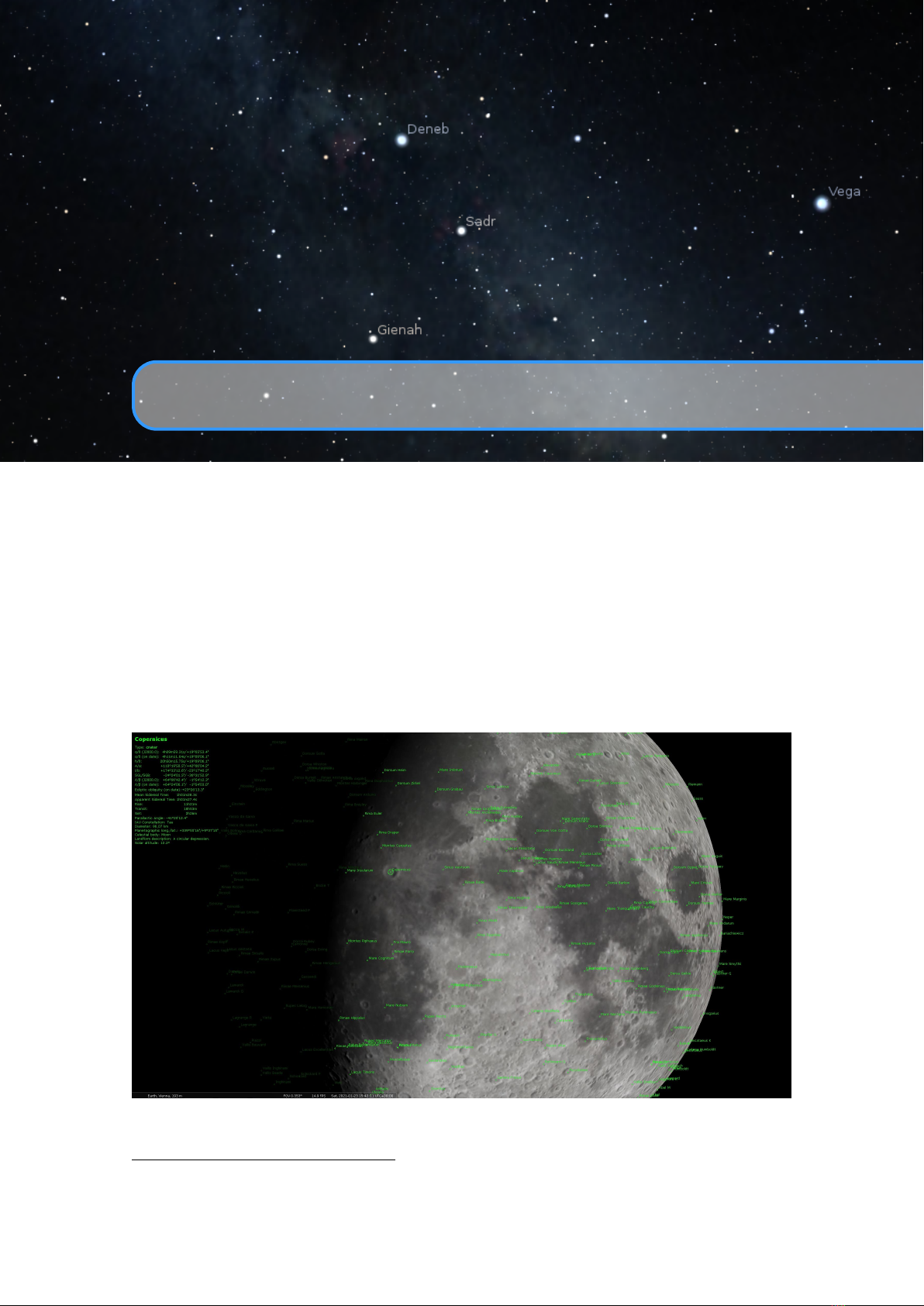
F.9 Comparison to Reference Data 399
Table F.2: An ephemeris comparison between Stellarium and JPL Horizons. Both are
showing geocentric apparent coordinates from the JPL DE440/441 ephemerides (with
slightly different models for precession, nutation and aberration; JPL results are also
corrected for light deflection). While results for present times agree very well, results
for the past seem to diverge a bit, presumably caused by differences in ∆T handling.
JPL Horizons (DE440/441) Stellarium 0.21.2β
UT Date Time RA J2000.0 DE J2000.0 α
J2000.0
δ
J2000.0
∆T
SUN
b2500-Jan-01 00:00
17h 24m 24.70s -23° 43’ 11.8” 17h 24m 23.52s -23° 43’ 13.2” 57938.45s
b2500-Jun-02 00:00
03h 06m 17.57s +17° 54’ 00.7” 03h 06m 16.61s +17° 53’ 58.6” 57927.29s
b2500-Nov-01 00:00
13h 11m 48.12s -07° 48’ 17.2” 13h 11m 47.07s -07° 48’ 11.5” 57916.12s
b2499-Apr-02 00:00
23h 26m 28.14s -03° 42’ 34.9” 23h 26m 27.30s -03° 42’ 40.9” 57904.96s
b0500-Jan-01 00:00
18h 25m 28.83s -23° 37’ 22.2” 18h 25m 28.82s -23° 37’ 23.4” 16704.77s
b0500-Jun-02 00:00
04h 09m 13.48s +21° 17’ 20.8” 04h 09m 13.50s +21° 17’ 21.9” 16698.78s
b0500-Nov-01 00:00
14h 04m 26.18s -12° 48’ 35.8” 14h 04m 26.15s -12° 48’ 36.3” 16692.79s
b0499-Apr-02 00:00
00h 21m 10.51s +02° 19’ 31.0” 00h 21m 10.52s +02° 19’ 31.1” 16686.79s
0500-Jan-01 00:00
18h 53m 06.08s -23° 04’ 11.0” 18h 53m 06.04s -23° 04’ 11.8” 5413.20s
0500-Jun-01 00:00
04h 39m 16.40s +22° 19’ 46.7” 04h 39m 16.39s +22° 19’ 47.4” 5409.79s
0500-Oct-31 00:00
14h 29m 26.81s -14° 52’ 19.2” 14h 29m 26.77s -14° 52’ 19.5” 5406.38s
0501-Apr-01 00:00
00h 46m 23.08s +05° 01’ 37.5” 00h 46m 23.07s +05° 01’ 37.6” 5402.97s
0501-Aug-31 00:00
10h 41m 17.14s +08° 22’ 56.8” 10h 41m 17.14s +08° 22’ 57.2” 5399.56s
1600-Jan-01 00:00
18h 43m 28.07s -23° 06’ 56.6” 18h 43m 28.33s -23° 06’ 56.5” 141.31s
1600-Jun-01 00:00
04h 35m 37.18s +22° 04’ 25.0” 04h 35m 37.43s +22° 04’ 25.6” 140.84s
1600-Oct-31 00:00
14h 21m 56.45s -14° 09’ 38.9” 14h 21m 56.68s -14° 09’ 40.1” 140.37s
1601-Apr-01 00:00
00h 41m 18.48s +04° 27’ 19.4” 00h 41m 18.70s +04° 27’ 20.8” 139.90s
1601-Aug-31 00:00
10h 36m 30.29s +08° 48’ 10.8” 10h 36m 30.52s +08° 48’ 09.6” 139.44s
2021-Jan-01 00:00
18h 46m 53.59s -22° 59’ 57.2” 18h 46m 53.59s -22° 59’ 57.2” 65.79s
2021-Jun-02 00:00
04h 40m 40.91s +22° 11’ 09.1” 04h 40m 40.90s +22° 11’ 09.1” 66.11s
2021-Nov-01 00:00
14h 25m 34.78s -14° 25’ 31.0” 14h 25m 34.78s -14° 25’ 30.9” 66.43s
2022-Apr-02 00:00
00h 45m 00.07s +04° 50’ 03.8” 00h 45m 00.07s +04° 50’ 03.7” 66.76s
MERCURY
b2500-Jan-01 00:00
17h 07m 28.00s -25° 22’ 36.2” 17h 07m 24.54s -25° 22’ 33.7” 57938.45s
b2500-Jun-02 00:00
04h 57m 29.05s +22° 59’ 25.2” 04h 57m 28.40s +22° 59’ 34.3” 57927.29s
b2500-Nov-01 00:00
11h 56m 15.20s +03° 10’ 47.5” 11h 56m 14.50s +03° 10’ 55.1” 57916.12s
b2499-Apr-02 00:00
23h 03m 07.53s -07° 14’ 26.7” 23h 03m 04.03s -07° 14’ 56.6” 57904.96s
b0500-Jan-01 00:00
18h 40m 28.21s -25° 26’ 38.0” 18h 40m 27.54s -25° 26’ 40.0” 16704.77s
b0500-Jun-02 00:00
05h 38m 48.42s +22° 19’ 54.2” 05h 38m 49.11s +22° 19’ 58.7” 16698.78s
b0500-Nov-01 00:00
12h 56m 45.19s -03° 57’ 14.5” 12h 56m 44.96s -03° 57’ 12.2” 16692.79s
b0499-Apr-02 00:00
00h 21m 09.78s +01° 53’ 27.6” 00h 21m 08.99s +01° 53’ 20.6” 16686.79s
0500-Jan-01 00:00
18h 23m 39.86s -25° 14’ 04.0” 18h 23m 39.46s -25° 14’ 04.4” 5413.20s
0500-Jun-01 00:00
06h 29m 34.30s +24° 32’ 58.8” 06h 29m 34.21s +24° 33’ 00.8” 5409.79s
0500-Oct-31 00:00
13h 28m 10.47s -06° 51’ 07.8” 13h 28m 10.93s -06° 51’ 11.8” 5406.38s
0501-Apr-01 00:00
23h 55m 15.72s -02° 45’ 50.1” 23h 55m 15.30s -02° 45’ 53.7” 5402.97s
0501-Aug-31 00:00
12h 03m 40.27s -01° 48’ 53.7” 12h 03m 40.10s -01° 48’ 51.4” 5399.56s
1600-Jan-01 00:00
19h 16m 55.37s -24° 27’ 04.8” 19h 16m 55.69s -24° 27’ 04.5” 141.31s
1600-Jun-01 00:00
05h 27m 00.75s +22° 06’ 49.9” 05h 27m 00.88s +22° 06’ 49.8” 140.84s
1600-Oct-31 00:00
13h 24m 30.87s -06° 45’ 17.1” 13h 24m 31.13s -06° 45’ 18.8” 140.37s
1601-Apr-01 00:00
00h 45m 30.34s +03° 58’ 05.0” 00h 45m 30.64s +03° 58’ 07.2” 139.90s
1601-Aug-31 00:00
12h 08m 26.65s -04° 19’ 14.8” 12h 08m 26.83s -04° 19’ 16.2” 139.44s
2021-Jan-01 00:00
19h 17m 59.43s -24° 20’ 58.1” 19h 17m 59.41s -24° 20’ 58.2” 65.79s
2021-Jun-02 00:00
05h 35m 35.59s +22° 40’ 50.7” 05h 35m 35.59s +22° 40’ 50.7” 66.11s
2021-Nov-01 00:00
13h 25m 55.55s -06° 47’ 18.8” 13h 25m 55.54s -06° 47’ 18.7” 66.43s
2022-Apr-02 00:00
00h 43m 05.35s +03° 21’ 44.7” 00h 43m 05.34s +03° 21’ 44.7” 66.76s
VENUS
b2500-Jan-01 00:00
14h 38m 40.01s -10° 33’ 46.3” 14h 38m 40.01s -10° 33’ 46.8” 57938.45s
b2500-Jun-02 00:00
01h 31m 36.91s +08° 30’ 50.3” 01h 31m 35.42s +08° 30’ 41.0” 57927.29s
b2500-Nov-01 00:00
14h 04m 33.57s -13° 23’ 07.7” 14h 04m 31.93s -13° 22’ 58.4” 57916.12s
b2499-Apr-02 00:00
02h 07m 22.90s +16° 14’ 49.7” 02h 07m 21.78s +16° 14’ 43.3” 57904.96s
b0500-Jan-01 00:00
15h 15m 48.26s -13° 58’ 19.4” 15h 15m 48.35s -13° 58’ 20.3” 16704.77s
b0500-Jun-02 00:00
02h 41m 50.72s +14° 49’ 02.0” 02h 41m 50.54s +14° 49’ 01.5” 16698.78s
b0500-Nov-01 00:00
15h 14m 41.57s -18° 52’ 17.3” 15h 14m 41.35s -18° 52’ 16.9” 16692.79s
b0499-Apr-02 00:00
03h 10m 27.71s +21° 27’ 17.2” 03h 10m 27.72s +21° 27’ 17.6” 16686.79s
0500-Jan-01 00:00
20h 18m 43.11s -15° 30’ 09.1” 20h 18m 43.83s -15° 30’ 09.4” 5413.20s
0500-Jun-01 00:00
02h 11m 10.44s +11° 10’ 10.0” 02h 11m 10.33s +11° 10’ 09.7” 5409.79s
0500-Oct-31 00:00
14h 33m 32.68s -14° 39’ 03.4” 14h 33m 32.50s -14° 39’ 02.8” 5406.38s
0501-Apr-01 00:00
03h 03m 13.09s +18° 47’ 05.5” 03h 03m 12.97s +18° 47’ 05.1” 5402.97s
0501-Aug-31 00:00
09h 10m 52.83s +08° 18’ 44.4” 09h 10m 53.44s +08° 18’ 40.8” 5399.56s
1600-Jan-01 00:00
17h 09m 26.57s -18° 08’ 55.1” 17h 09m 26.71s -18° 08’ 55.3” 141.31s
1600-Jun-01 00:00
02h 28m 53.12s +12° 50’ 48.1” 02h 28m 53.37s +12° 50’ 49.4” 140.84s
1600-Oct-31 00:00
14h 54m 13.53s -16° 15’ 03.3” 14h 54m 13.79s -16° 15’ 04.6” 140.37s
1601-Apr-01 00:00
03h 18m 37.64s +20° 06’ 01.5” 03h 18m 37.90s +20° 06’ 02.6” 139.90s
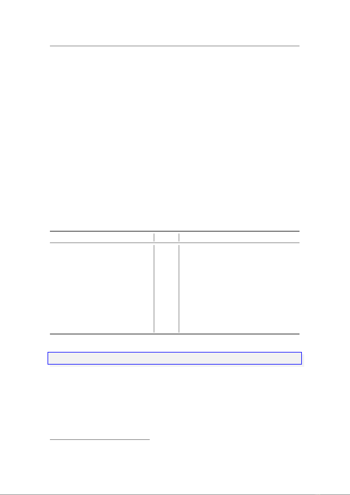
400 Appendix F. Accuracy
JPL Horizons (DE440/441) Stellarium 0.21.2β
UT Date Time RA J2000.0 DE J2000.0 α
J2000.0
δ
J2000.0
∆T
1601-Aug-31 00:00 07h 48m 52.93s +16° 06’ 13.5” 07h 48m 53.14s +16° 06’ 13.3” 139.44s
2021-Jan-01 00:00
17h 18m 28.43s -22° 26’ 01.6” 17h 18m 28.42s -22° 26’ 01.5” 65.79s
2021-Jun-02 00:00
05h 57m 01.46s +24° 21’ 39.2” 05h 57m 01.45s +24° 21’ 39.2” 66.11s
2021-Nov-01 00:00
17h 40m 41.73s -27° 05’ 05.3” 17h 40m 41.73s -27° 05’ 05.3” 66.43s
2022-Apr-02 00:00
21h 52m 25.36s -12° 04’ 41.5” 21h 52m 25.35s -12° 04’ 41.5” 66.76s
MOON
b2500-Jan-01 00:00
00h 13m 40.60s -00° 43’ 59.3” 00h 13m 13.41s -00° 47’ 44.2” 57938.45s
b2500-Jun-02 00:00
12h 48m 51.83s -04° 50’ 11.6” 12h 48m 20.00s -04° 45’ 50.3” 57927.29s
b2500-Nov-01 00:00
02h 49m 20.95s +19° 57’ 17.4” 02h 48m 49.83s +19° 54’ 22.0” 57916.12s
b2499-Apr-02 00:00
15h 45m 48.47s -25° 00’ 31.4” 15h 45m 11.61s -24° 58’ 11.1” 57904.96s
b0500-Jan-01 00:00
02h 14m 28.99s +14° 10’ 37.4” 02h 14m 20.11s +14° 10’ 05.8” 16704.77s
b0500-Jun-02 00:00
15h 02m 34.83s -16° 05’ 08.5” 15h 02m 24.07s -16° 04’ 39.3” 16698.78s
b0500-Nov-01 00:00
05h 18m 41.70s +19° 00’ 42.7” 05h 18m 32.17s +19° 00’ 41.6” 16692.79s
b0499-Apr-02 00:00
18h 10m 41.75s -18° 33’ 49.1” 18h 10m 31.22s -18° 33’ 56.3” 16686.79s
0500-Jan-01 00:00
05h 33m 09.71s +28° 18’ 25.7” 05h 33m 02.93s +28° 18’ 25.0” 5413.20s
0500-Jun-01 00:00
19h 39m 46.24s -24° 36’ 20.7” 19h 39m 38.25s -24° 36’ 48.8” 5409.79s
0500-Oct-31 00:00
08h 41m 09.22s +19° 42’ 14.7” 08h 41m 03.32s +19° 42’ 46.3” 5406.38s
0501-Apr-01 00:00
22h 26m 23.71s -07° 51’ 05.2” 22h 26m 17.20s -07° 51’ 54.1” 5402.97s
0501-Aug-31 00:00
11h 28m 24.37s -00° 41’ 25.5” 11h 28m 19.05s -00° 40’ 44.2” 5399.56s
1600-Jan-01 00:00
07h 04m 55.02s +24° 04’ 37.3” 07h 04m 56.39s +24° 04’ 33.9” 141.31s
1600-Jun-01 00:00
19h 54m 15.59s -20° 26’ 36.3” 19h 54m 16.89s -20° 26’ 31.4” 140.84s
1600-Oct-31 00:00
10h 11m 24.53s +07° 13’ 09.4” 10h 11m 25.66s +07° 13’ 02.2” 140.37s
1601-Apr-01 00:00
22h 46m 21.63s -02° 54’ 30.7” 22h 46m 22.87s -02° 54’ 22.4” 139.90s
1601-Aug-31 00:00
12h 52m 10.20s -10° 52’ 36.0” 12h 52m 11.39s -10° 52’ 43.0” 139.44s
2021-Jan-01 00:00
08h 23m 36.67s +23° 01’ 21.2” 08h 23m 36.54s +23° 01’ 21.5” 65.79s
2021-Jun-02 00:00
22h 46m 54.03s -13° 27’ 21.8” 22h 46m 53.93s -13° 27’ 22.4” 66.11s
2021-Nov-01 00:00
11h 18m 43.58s +09° 57’ 42.8” 11h 18m 43.49s +09° 57’ 43.4” 66.43s
2022-Apr-02 00:00
01h 21m 51.21s +05° 40’ 00.7” 01h 21m 51.14s +05° 40’ 00.1” 66.76s
MARS
1601-Jan-01 00:00
19h 26m 56.21s -23° 01’ 42.7” 19h 26m 56.45s -23° 01’ 42.4” 140.18s
1601-Jun-02 00:00
02h 59m 06.93s +16° 41’ 21.5” 02h 59m 07.15s +16° 41’ 22.6” 139.71s
1601-Nov-01 00:00
09h 48m 48.55s +15° 01’ 38.0” 09h 48m 48.75s +15° 01’ 37.2” 139.25s
1602-Apr-02 00:00
10h 25m 38.57s +13° 17’ 29.7” 10h 25m 38.70s +13° 17’ 29.0” 138.78s
2021-Jan-01 00:00
01h 40m 18.14s +11° 20’ 41.2” 01h 40m 18.14s +11° 20’ 41.1” 65.79s
2021-Jun-02 00:00
07h 45m 03.73s +22° 37’ 21.0” 07h 45m 03.72s +22° 37’ 21.0” 66.11s
2021-Nov-01 00:00
13h 55m 54.00s -11° 22’ 08.1” 13h 55m 54.00s -11° 22’ 08.1” 66.43s
2022-Apr-02 00:00
21h 31m 33.53s -15° 56’ 58.5” 21h 31m 33.53s -15° 56’ 58.5” 66.76s
JUPITER
1601-Jan-01 00:00
11h 33m 23.43s +04° 18’ 09.3” 11h 33m 23.58s +04° 18’ 08.4” 140.18s
1601-Jun-02 00:00
10h 59m 49.52s +07° 52’ 18.0” 10h 59m 49.67s +07° 52’ 17.1” 139.71s
1601-Nov-01 00:00
12h 39m 41.32s -03° 02’ 14.3” 12h 39m 41.47s -03° 02’ 15.3” 139.25s
1602-Apr-02 00:00
13h 08m 44.17s -05° 35’ 33.6” 13h 08m 44.30s -05° 35’ 34.4” 138.78s
2021-Jan-01 00:00
20h 20m 44.62s -20° 00’ 44.3” 20h 20m 44.62s -20° 00’ 44.4” 65.79s
2021-Jun-02 00:00
22h 15m 51.65s -11° 42’ 45.3” 22h 15m 51.65s -11° 42’ 45.3” 66.11s
2021-Nov-01 00:00
21h 41m 29.27s -15° 01’ 08.9” 21h 41m 29.27s -15° 01’ 08.9” 66.43s
2022-Apr-02 00:00
23h 30m 29.23s -04° 17’ 08.2” 23h 30m 29.24s -04° 17’ 08.2” 66.76s
SATURN
1750-Jan-01 00:00
15h 46m 12.27s -17° 54’ 37.7” 15h 46m 12.37s -17° 54’ 38.1” 22.71s
1750-Jun-02 00:00
15h 44m 23.78s -17° 34’ 00.9” 15h 44m 23.87s -17° 34’ 01.3” 22.52s
1750-Nov-01 00:00
15h 59m 19.00s -18° 50’ 41.0” 15h 59m 19.10s -18° 50’ 41.4” 22.34s
1751-Apr-02 00:00
16h 49m 11.72s -20° 39’ 30.2” 16h 49m 11.82s -20° 39’ 30.5” 22.15s
2021-Jan-01 00:00
20h 15m 50.41s -20° 10’ 28.7” 20h 15m 50.41s -20° 10’ 28.7” 65.79s
2021-Jun-02 00:00
21h 04m 25.24s -17° 24’ 46.6” 21h 04m 25.24s -17° 24’ 46.6” 66.11s
2021-Nov-01 00:00
20h 39m 27.72s -19° 14’ 59.7” 20h 39m 27.72s -19° 14’ 59.7” 66.43s
2022-Apr-02 00:00
21h 39m 14.50s -15° 01’ 42.2” 21h 39m 14.50s -15° 01’ 42.2” 66.76s
URANUS
1600-Jan-01 00:00
01h 41m 51.34s +10° 01’ 26.1” 01h 41m 51.49s +10° 01’ 26.9” 141.31s
1600-Jun-01 00:00
02h 05m 21.58s +12° 13’ 45.6” 02h 05m 21.73s +12° 13’ 46.4” 140.84s
1600-Oct-31 00:00
02h 04m 09.95s +12° 05’ 39.9” 02h 04m 10.09s +12° 05’ 40.7” 140.37s
1601-Apr-01 00:00
02h 07m 08.63s +12° 25’ 31.5” 02h 07m 08.78s +12° 25’ 32.4” 139.90s
1601-Aug-31 00:00
02h 28m 09.10s +14° 11’ 23.3” 02h 28m 09.24s +14° 11’ 24.1” 139.44s
2021-Jan-01 00:00
02h 18m 27.82s +13° 21’ 27.5” 02h 18m 27.83s +13° 21’ 27.5” 65.79s
2021-Jun-02 00:00
02h 40m 37.83s +15° 11’ 44.7” 02h 40m 37.84s +15° 11’ 44.7” 66.11s
2021-Nov-01 00:00
02h 42m 31.60s +15° 19’ 13.5” 02h 42m 31.60s +15° 19’ 13.5” 66.43s
2022-Apr-02 00:00
02h 42m 25.31s +15° 22’ 19.7” 02h 42m 25.31s +15° 22’ 19.7” 66.76s
NEPTUNE
1801-Jan-01 00:00
15h 07m 04.41s -15° 44’ 47.2” 15h 07m 04.49s -15° 44’ 47.6” 5.51s
1801-Jun-02 00:00
15h 01m 57.08s -15° 18’ 05.9” 15h 01m 57.15s -15° 18’ 06.2” 5.42s
1801-Nov-01 00:00
15h 07m 02.36s -15° 46’ 26.5” 15h 07m 02.43s -15° 46’ 26.9” 5.33s
1802-Apr-02 00:00
15h 17m 01.46s -16° 20’ 15.8” 15h 17m 01.54s -16° 20’ 16.2” 5.24s

F.9 Comparison to Reference Data 401
JPL Horizons (DE440/441) Stellarium 0.21.2β
UT Date Time RA J2000.0 DE J2000.0 α
J2000.0
δ
J2000.0
∆T
2021-Jan-01 00:00 23h 19m 18.38s -05° 33’ 12.4” 23h 19m 18.39s -05° 33’ 12.4” 65.79s
2021-Jun-02 00:00
23h 36m 13.26s -03° 46’ 42.9” 23h 36m 13.26s -03° 46’ 42.9” 66.11s
2021-Nov-01 00:00
23h 27m 30.35s -04° 46’ 19.7” 23h 27m 30.35s -04° 46’ 19.7” 66.43s
2022-Apr-02 00:00
23h 38m 17.59s -03° 34’ 19.0” 23h 38m 17.59s -03° 34’ 19.0” 66.76s
IO(JI)
1601-Jan-01 00:00
11h 33m 30.36s +04° 17’ 19.7” 11h 33m 30.51s +04° 17’ 18.9” 140.18s
1601-Jun-02 00:00
10h 59m 55.45s +07° 51’ 35.7” 10h 59m 55.61s +07° 51’ 34.8” 139.71s
1601-Nov-01 00:00
12h 39m 41.63s -03° 02’ 20.8” 12h 39m 41.81s -03° 02’ 22.0” 139.25s
1602-Apr-02 00:00
13h 08m 39.94s -05° 35’ 12.3” 13h 08m 40.11s -05° 35’ 13.4” 138.78s
2021-Jan-01 00:00
20h 20m 41.43s -20° 00’ 57.7” 20h 20m 41.43s -20° 00’ 57.7” 65.79s
2021-Jun-02 00:00
22h 15m 44.01s -11° 43’ 33.2” 22h 15m 44.01s -11° 43’ 33.2” 66.11s
2021-Nov-01 00:00
21h 41m 21.65s -15° 01’ 52.3” 21h 41m 21.65s -15° 01’ 52.3” 66.43s
2022-Apr-02 00:00
23h 30m 27.92s -04° 17’ 20.4” 23h 30m 27.93s -04° 17’ 20.4” 66.76s
EUROPA(JII)
1601-Jan-01 00:00
11h 33m 16.17s +04° 19’ 07.1” 11h 33m 16.29s +04° 19’ 06.3” 140.18s
1601-Jun-02 00:00
10h 59m 53.24s +07° 51’ 59.3” 10h 59m 53.37s +07° 51’ 58.7” 139.71s
1601-Nov-01 00:00
12h 39m 49.09s -03° 03’ 11.4” 12h 39m 49.26s -03° 03’ 12.3” 139.25s
1602-Apr-02 00:00
13h 08m 40.13s -05° 35’ 20.4” 13h 08m 40.28s -05° 35’ 21.3” 138.78s
2021-Jan-01 00:00
20h 20m 34.16s -20° 01’ 24.9” 20h 20m 34.16s -20° 01’ 24.9” 65.79s
2021-Jun-02 00:00
22h 15m 55.57s -11° 42’ 23.5” 22h 15m 55.57s -11° 42’ 23.5” 66.11s
2021-Nov-01 00:00
21h 41m 41.68s -14° 59’ 58.2” 21h 41m 41.68s -14° 59’ 58.2” 66.43s
2022-Apr-02 00:00
23h 30m 29.10s -04° 17’ 03.2” 23h 30m 29.11s -04° 17’ 03.3” 66.76s
GANYMEDE(JIII)
1601-Jan-01 00:00
11h 33m 29.35s +04° 17’ 17.1” 11h 33m 29.49s +04° 17’ 16.2” 140.18s
1601-Jun-02 00:00
11h 00m 04.63s +07° 50’ 38.0” 11h 00m 04.78s +07° 50’ 37.2” 139.71s
1601-Nov-01 00:00
12h 39m 41.91s -03° 02’ 07.8” 12h 39m 42.07s -03° 02’ 08.7” 139.25s
1602-Apr-02 00:00
13h 08m 24.28s -05° 33’ 17.7” 13h 08m 24.40s -05° 33’ 18.6” 138.78s
2021-Jan-01 00:00
20h 20m 33.16s -20° 01’ 30.9” 20h 20m 33.15s -20° 01’ 30.9” 65.79s
2021-Jun-02 00:00
22h 15m 57.19s -11° 42’ 07.4” 22h 15m 57.19s -11° 42’ 07.5” 66.11s
2021-Nov-01 00:00
21h 41m 47.81s -14° 59’ 25.0” 21h 41m 47.82s -14° 59’ 25.0” 66.43s
2022-Apr-02 00:00
23h 30m 31.22s -04° 17’ 01.0” 23h 30m 31.23s -04° 17’ 01.0” 66.76s
CALLISTO(JIV)
1601-Jan-01 00:00
11h 33m 15.59s +04° 19’ 21.5” 11h 33m 15.73s +04° 19’ 20.6” 140.18s
1601-Jun-02 00:00
10h 59m 22.98s +07° 55’ 21.8” 10h 59m 23.12s +07° 55’ 20.9” 139.71s
1601-Nov-01 00:00
12h 39m 17.32s -02° 59’ 27.6” 12h 39m 17.47s -02° 59’ 28.8” 139.25s
1602-Apr-02 00:00
13h 08m 09.98s -05° 32’ 01.2” 13h 08m 10.10s -05° 32’ 02.1” 138.78s
2021-Jan-01 00:00
20h 20m 42.72s -20° 00’ 56.3” 20h 20m 42.73s -20° 00’ 56.3” 65.79s
2021-Jun-02 00:00
22h 15m 55.40s -11° 42’ 15.1” 22h 15m 55.41s -11° 42’ 15.1” 66.11s
2021-Nov-01 00:00
21h 41m 58.24s -14° 58’ 23.9” 21h 41m 58.25s -14° 58’ 23.9” 66.43s
2022-Apr-02 00:00
23h 30m 53.15s -04° 14’ 15.0” 23h 30m 53.15s -04° 14’ 15.0” 66.76s
Table F.3: An ephemeris comparison between Stellarium and JPL Horizons, based on JPL
DE440/441. Both are showing geocentric apparent coordinates (with slightly different
models for precession, nutation and aberration; JPL results are also corrected for light
deflection). This table shows ephemeris comparison in Dynamical time (TT), to avoid
showing divergences which are only caused by differences in
∆T
handling. (JPL’s values
for ∆T are listed for reference, but not used.)
JPL Horizons Stellarium 0.21.2β
TT Date Time RA J2000.0 DE J2000.0 ∆T α
J2000.0
δ
J2000.0
SUN
b2500-Jan-01 00:00
17h21m25.18s -23°40’30.1” 58893.015756s 17h21m26.91s -23°40’34.2”
b2500-Jun-02 00:00
03h03m40.51s +17°43’04.0” 58881.693980s 03h03m42.09s +17°43’12.5”
b2500-Nov-01 00:00
13h09m12.65s -07°32’06.5” 58870.373294s 13h09m14.12s -07°32’16.5”
b2499-Apr-02 00:00
23h24m04.53s -03°58’17.6” 58859.053698s 23h24m06.02s -03°58’08.4”
b0500-Jan-01 00:00
18h24m36.63s -23°37’53.7” 16988.259557s 18h24m37.49s -23°37’54.4”
b0500-Jun-02 00:00
04h08m26.19s +21°15’14.4” 16982.002779s 04h08m26.99s +21°15’17.6”
b0500-Nov-01 00:00
14h03m40.03s -12°44’27.5” 16975.747099s 14h03m40.76s -12°44’32.1”
b0499-Apr-02 00:00
00h20m28.76s +02°14’57.0” 16969.492518s 00h20m29.48s +02°15’01.7”
0500-Jan-01 00:00
18h52m48.93s -23°04’32.9” 5608.981515s 18h52m49.49s -23°04’32.9”
0500-Jun-01 00:00
04h39m00.52s +22°19’15.9” 5605.028887s 04h39m01.07s +22°19’17.7”
0500-Oct-31 00:00
14h29m11.35s -14°51’03.8” 5601.076499s 14h29m11.84s -14°51’06.7”
0501-Apr-01 00:00
00h46m09.14s +05°00’08.5” 5597.124355s 00h46m09.61s +05°00’11.6”
0501-Aug-31 00:00
10h41m02.87s +08°24’23.2” 5593.172456s 10h41m03.36s +08°24’20.5”
1600-Jan-01 00:00
18h43m27.73s -23°06’56.9” 110.462079s 18h43m27.90s -23°06’57.0”
1600-Jun-01 00:00
04h35m36.87s +22°04’24.3” 109.804702s 04h35m37.03s +22°04’24.8”
1600-Oct-31 00:00
14h21m56.15s -14°09’37.4” 109.148794s 14h21m56.30s -14°09’38.2”
1601-Apr-01 00:00
00h41m18.21s +04°27’17.7” 108.494367s 00h41m18.35s +04°27’18.6”

402 Appendix F. Accuracy
JPL Horizons Stellarium 0.21.2β
TT Date Time RA J2000.0 DE J2000.0 ∆T α
J2000.0
δ
J2000.0
1601-Aug-31 00:00 10h36m30.02s +08°48’12.4” 107.841429s 10h36m30.16s +08°48’11.7”
MERCURY
b2500-Jan-01 00:00
17h02m08.10s -25°14’54.4” 58893.015756s 17h02m09.83s -25°14’59.3”
b2500-Jun-02 00:00
04h55m00.41s +23°03’30.5” 58881.693980s 04h55m02.12s +23°03’35.5”
b2500-Nov-01 00:00
11h54m04.49s +03°27’59.5” 58870.373294s 11h54m05.97s +03°27’49.8”
b2499-Apr-02 00:00
22h57m59.14s -07°54’02.4” 58859.053698s 22h58m00.66s -07°53’53.6”
b0500-Jan-01 00:00
18h38m56.17s -25°28’13.0” 16988.259557s 18h38m57.04s -25°28’13.3”
b0500-Jun-02 00:00
05h38m38.91s +22°22’48.0” 16982.002779s 05h38m39.75s +22°22’49.6”
b0500-Nov-01 00:00
12h55m48.65s -03°50’09.1” 16975.747099s 12h55m49.37s -03°50’13.9”
b0499-Apr-02 00:00
00h19m39.97s +01°41’26.3” 16969.492518s 00h19m40.68s +01°41’31.2”
0500-Jan-01 00:00
18h23m11.76s -25°14’05.2” 5608.981515s 18h23m12.34s -25°14’05.6”
0500-Jun-01 00:00
06h29m15.56s +24°33’46.9” 5605.028887s 06h29m16.13s +24°33’47.2”
0500-Oct-31 00:00
13h28m09.82s -06°51’31.3” 5601.076499s 13h28m10.29s -06°51’34.4”
0501-Apr-01 00:00
23h54m49.90s -02°49’01.2” 5597.124355s 23h54m50.38s -02°48’58.1”
0501-Aug-31 00:00
12h03m21.92s -01°46’20.3” 5593.172456s 12h03m22.39s -01°46’23.4”
1600-Jan-01 00:00
19h16m54.82s -24°27’05.8” 110.462079s 19h16m54.99s -24°27’05.7”
1600-Jun-01 00:00
05h27m00.83s +22°06’51.2” 109.804702s 05h27m01.00s +22°06’51.5”
1600-Oct-31 00:00
13h24m30.45s -06°45’14.3” 109.148794s 13h24m30.59s -06°45’15.2”
1601-Apr-01 00:00
00h45m29.79s +03°58’00.7” 108.494367s 00h45m29.92s +03°58’01.7”
1601-Aug-31 00:00
12h08m26.49s -04°19’13.1” 107.841429s 12h08m26.63s -04°19’14.0”
VENUS
b2500-Jan-01 00:00
14h37m07.30s -10°25’08.5” 58893.015756s 14h37m08.81s -10°25’17.6”
b2500-Jun-02 00:00
01h28m34.06s +08°11’02.7” 58881.693980s 01h28m35.54s +08°11’12.6”
b2500-Nov-01 00:00
14h01m18.60s -13°03’41.8” 58870.373294s 14h01m20.11s -13°03’51.3”
b2499-Apr-02 00:00
02h04m39.28s +15°58’24.8” 58859.053698s 02h04m40.81s +15°58’34.2”
b0500-Jan-01 00:00
15h15m08.22s -13°55’20.5” 16988.259557s 15h15m08.98s -13°55’24.4”
b0500-Jun-02 00:00
02h40m55.02s +14°44’15.5” 16982.002779s 02h40m55.77s +14°44’19.8”
b0500-Nov-01 00:00
15h13m42.04s -18°47’53.8” 16975.747099s 15h13m42.82s -18°47’57.7”
b0499-Apr-02 00:00
03h09m40.90s +21°23’39.0” 16969.492518s 03h09m41.68s +21°23’43.0”
0500-Jan-01 00:00
20h18m48.52s -15°30’50.9” 5608.981515s 20h18m49.05s -15°30’49.8”
0500-Jun-01 00:00
02h10m53.15s +11°08’35.0” 5605.028887s 02h10m53.64s +11°08’38.0”
0500-Oct-31 00:00
14h33m13.65s -14°37’22.9” 5601.076499s 14h33m14.14s -14°37’25.8”
0501-Apr-01 00:00
03h02m54.73s +18°45’37.5” 5597.124355s 03h02m55.25s +18°45’40.1”
0501-Aug-31 00:00
09h10m56.37s +08°17’52.4” 5593.172456s 09h10m56.87s +08°17’50.6”
1600-Jan-01 00:00
17h09m26.64s -18°08’55.7” 110.462079s 17h09m26.80s -18°08’56.1”
1600-Jun-01 00:00
02h28m52.77s +12°50’46.3” 109.804702s 02h28m52.92s +12°50’47.1”
1600-Oct-31 00:00
14h54m13.16s -16°15’01.5” 109.148794s 14h54m13.31s -16°15’02.3”
1601-Apr-01 00:00
03h18m37.29s +20°05’59.9” 108.494367s 03h18m37.45s +20°06’00.6”
1601-Aug-31 00:00
07h48m52.75s +16°06’13.4” 107.841429s 07h48m52.90s +16°06’13.2”
MOON
b2500-Jan-01 00:00
23h43m54.13s -04°46’15.6” 58893.015756s 23h43m55.61s -04°46’06.1”
b2500-Jun-02 00:00
12h15m08.68s -00°12’02.6” 58881.693980s 12h15m10.14s -00°12’12.5”
b2500-Nov-01 00:00
02h16m07.77s +16°35’31.3” 58870.373294s 02h16m09.31s +16°35’40.6”
b2499-Apr-02 00:00
15h07m11.31s -22°11’27.1” 58859.053698s 15h07m12.93s -22°11’35.4”
b0500-Jan-01 00:00
02h04m52.71s +13°33’43.2” 16988.259557s 02h04m53.45s +13°33’47.8”
b0500-Jun-02 00:00
14h51m07.34s -15°30’50.9” 16982.002779s 14h51m08.09s -15°30’55.1”
b0500-Nov-01 00:00
05h08m19.28s +18°56’30.3” 16975.747099s 05h08m20.10s +18°56’32.5”
b0499-Apr-02 00:00
17h59m21.65s -18°38’44.9” 16969.492518s 17h59m22.47s -18°38’46.1”
0500-Jan-01 00:00
05h29m38.64s +28°17’23.7” 5608.981515s 05h29m39.22s +28°17’24.9”
0500-Jun-01 00:00
19h35m39.76s -24°49’55.2” 5605.028887s 19h35m40.33s -24°49’54.6”
0500-Oct-31 00:00
08h38m03.41s +19°57’58.9” 5601.076499s 08h38m03.95s +19°57’57.5”
0501-Apr-01 00:00
22h23m01.61s -08°15’47.6” 5597.124355s 22h23m02.11s -08°15’45.1”
0501-Aug-31 00:00
11h25m37.06s -00°20’06.1” 5593.172456s 11h25m37.53s -00°20’09.0”
1600-Jan-01 00:00
07h04m50.63s +24°04’49.5” 110.462079s 07h04m50.78s +24°04’49.4”
1600-Jun-01 00:00
19h54m11.52s -20°26’52.9” 109.804702s 19h54m11.67s -20°26’52.7”
1600-Oct-31 00:00
10h11m21.07s +07°13’32.6” 109.148794s 10h11m21.20s +07°13’32.0”
1601-Apr-01 00:00
22h46m17.79s -02°54’56.8” 108.494367s 22h46m17.91s -02°54’56.1”
1601-Aug-31 00:00
12h52m06.59s -10°52’15.0” 107.841429s 12h52m06.72s -10°52’15.8”
MARS
1601-Jan-01 00:00
19h26m55.96s -23°01’43.2” 108.881677s 19h26m56.12s -23°01’43.1”
1601-Jun-02 00:00
02h59m06.71s +16°41’20.6” 108.227856s 02h59m06.87s +16°41’21.3”
1601-Nov-01 00:00
09h48m48.40s +15°01’38.7” 107.575530s 09h48m48.55s +15°01’38.1”
1602-Apr-02 00:00
10h25m38.61s +13°17’29.7” 106.924708s 10h25m38.76s +13°17’28.9”
JUPITER
1601-Jan-01 00:00
11h33m23.43s +04°18’09.3” 108.881677s 11h33m23.57s +04°18’08.4”
1601-Jun-02 00:00
10h59m49.50s +07°52’18.1” 108.227856s 10h59m49.64s +07°52’17.3”
1601-Nov-01 00:00
12h39m41.26s -03°02’14.0” 107.575530s 12h39m41.40s -03°02’14.9”
1602-Apr-02 00:00
13h08m44.21s -05°35’33.8” 106.924708s 13h08m44.34s -05°35’34.7”
SATURN
1750-Jan-01 00:00 15h46m12.26s -17°54’37.7” 17.322273s 15h46m12.36s -17°54’38.1”

F.9 Comparison to Reference Data 403
JPL Horizons Stellarium 0.21.2β
TT Date Time RA J2000.0 DE J2000.0 ∆T α
J2000.0
δ
J2000.0
1750-Jun-02 00:00 15h44m23.78s -17°34’00.9” 17.413029s 15h44m23.88s -17°34’01.3”
1750-Nov-01 00:00
15h59m18.99s -18°50’41.0” 17.503706s 15h59m19.09s -18°50’41.4”
1751-Apr-02 00:00
16h49m11.73s -20°39’30.2” 17.594270s 16h49m11.82s -20°39’30.5”
URANUS
1600-Jan-01 00:00
01h41m51.35s +10°01’26.1” 110.462079s 01h41m51.49s +10°01’26.9”
1600-Jun-01 00:00
02h05m21.56s +12°13’45.5” 109.804702s 02h05m21.71s +12°13’46.3”
1600-Oct-31 00:00
02h04m09.96s +12°05’40.0” 109.148794s 02h04m10.11s +12°05’40.8”
1601-Apr-01 00:00
02h07m08.61s +12°25’31.4” 108.494367s 02h07m08.76s +12°25’32.3”
1601-Aug-31 00:00
02h28m09.10s +14°11’23.3” 107.841429s 02h28m09.25s +14°11’24.1”
NEPTUNE
1801-Jan-01 00:00
15h07m04.41s -15°44’47.2” 18.261920s 15h07m04.49s -15°44’47.6”
1801-Jun-02 00:00
15h01m57.08s -15°18’05.9” 18.107889s 15h01m57.15s -15°18’06.3”
1801-Nov-01 00:00
15h07m02.35s -15°46’26.5” 17.952783s 15h07m02.43s -15°46’26.9”
1802-Apr-02 00:00
15h17m01.46s -16°20’15.8” 17.797431s 15h17m01.54s -16°20’16.2”
IO(JI)
1601-Jan-01 00:00
11h33m30.35s +04°17’19.8” 108.881677s 11h33m30.50s +04°17’18.9”
1601-Jun-02 00:00
10h59m55.42s +07°51’35.9” 108.227856s 10h59m55.57s +07°51’35.0”
1601-Nov-01 00:00
12h39m41.55s -03°02’20.3” 107.575530s 12h39m41.71s -03°02’21.4”
1602-Apr-02 00:00
13h08m39.95s -05°35’12.3” 106.924708s 13h08m40.11s -05°35’13.4”
EUROPA(JII)
1601-Jan-01 00:00
11h33m16.18s +04°19’07.0” 108.881677s 11h33m16.31s +04°19’06.2”
1601-Jun-02 00:00
10h59m53.24s +07°51’59.3” 108.227856s 10h59m53.38s +07°51’58.6”
1601-Nov-01 00:00
12h39m49.02s -03°03’11.0” 107.575530s 12h39m49.17s -03°03’11.8”
1602-Apr-02 00:00
13h08m40.14s -05°35’20.5” 106.924708s 13h08m40.29s -05°35’21.4”
GANYMEDE(JIII)
1601-Jan-01 00:00
11h33m29.32s +04°17’17.3” 108.881677s 11h33m29.46s +04°17’16.4”
1601-Jun-02 00:00
11h00m04.62s +07°50’38.1” 108.227856s 11h00m04.77s +07°50’37.3”
1601-Nov-01 00:00
12h39m41.87s -03°02’07.5” 107.575530s 12h39m42.01s -03°02’08.4”
1602-Apr-02 00:00
13h08m24.32s -05°33’17.9” 106.924708s 13h08m24.46s -05°33’18.9”
CALLISTO(JIV)
1601-Jan-01 00:00
11h33m15.60s +04°19’21.4” 108.881677s 11h33m15.74s +04°19’20.5”
1601-Jun-02 00:00
10h59m22.96s +07°55’21.9” 108.227856s 10h59m23.10s +07°55’21.0”
1601-Nov-01 00:00
12h39m17.27s -02°59’27.3” 107.575530s 12h39m17.41s -02°59’28.3”
1602-Apr-02 00:00
13h08m10.01s -05°32’01.4” 106.924708s 13h08m10.14s -05°32’02.4”

G. GNU Free Documentation License
Version 1.3, 3 November 2008
Copyright © 2000, 2001, 2002, 2007, 2008 Free Software Foundation, Inc. http://fsf.org/
Everyone is permitted to copy and distribute verbatim copies of this license document, but changing
it is not allowed.
G.1 PREAMBLE
The purpose of this License is to make a manual, textbook, or other functional and useful document
“free” in the sense of freedom: to assure everyone the effective freedom to copy and redistribute it,
with or without modifying it, either commercially or noncommercially. Secondarily, this License
preserves for the author and publisher a way to get credit for their work, while not being considered
responsible for modifications made by others.
This License is a kind of “copyleft”, which means that derivative works of the document must
themselves be free in the same sense. It complements the GNU General Public License, which is a
copyleft license designed for free software.
We have designed this License in order to use it for manuals for free software, because free
software needs free documentation: a free program should come with manuals providing the same
freedoms that the software does. But this License is not limited to software manuals; it can be used
for any textual work, regardless of subject matter or whether it is published as a printed book. We
recommend this License principally for works whose purpose is instruction or reference.
G.2 APPLICABILITY AND DEFINITIONS
This License applies to any manual or other work, in any medium, that contains a notice placed by
the copyright holder saying it can be distributed under the terms of this License. Such a notice grants
a world-wide, royalty-free license, unlimited in duration, to use that work under the conditions
stated herein. The “Document”, below, refers to any such manual or work. Any member of the
public is a licensee, and is addressed as “you”. You accept the license if you copy, modify or
distribute the work in a way requiring permission under copyright law.
A “Modified Version” of the Document means any work containing the Document or a portion
of it, either copied verbatim, or with modifications and/or translated into another language.
A “Secondary Section” is a named appendix or a front-matter section of the Document that deals
exclusively with the relationship of the publishers or authors of the Document to the Document’s
overall subject (or to related matters) and contains nothing that could fall directly within that overall
406 Appendix G. GNU Free Documentation License
subject. (Thus, if the Document is in part a textbook of mathematics, a Secondary Section may
not explain any mathematics.) The relationship could be a matter of historical connection with the
subject or with related matters, or of legal, commercial, philosophical, ethical or political position
regarding them.
The “Invariant Sections” are certain Secondary Sections whose titles are designated, as being
those of Invariant Sections, in the notice that says that the Document is released under this License.
If a section does not fit the above definition of Secondary then it is not allowed to be designated as
Invariant. The Document may contain zero Invariant Sections. If the Document does not identify
any Invariant Sections then there are none.
The “Cover Texts” are certain short passages of text that are listed, as Front-Cover Texts or
Back-Cover Texts, in the notice that says that the Document is released under this License. A
Front-Cover Text may be at most 5 words, and a Back-Cover Text may be at most 25 words.
A “Transparent” copy of the Document means a machine-readable copy, represented in a
format whose specification is available to the general public, that is suitable for revising the
document straightforwardly with generic text editors or (for images composed of pixels) generic
paint programs or (for drawings) some widely available drawing editor, and that is suitable for
input to text formatters or for automatic translation to a variety of formats suitable for input to
text formatters. A copy made in an otherwise Transparent file format whose markup, or absence
of markup, has been arranged to thwart or discourage subsequent modification by readers is not
Transparent. An image format is not Transparent if used for any substantial amount of text. A copy
that is not “Transparent” is called “Opaque”.
Examples of suitable formats for Transparent copies include plain ASCII without markup,
Texinfo input format, LaTeX input format, SGML or XML using a publicly available DTD, and
standard-conforming simple HTML, PostScript or PDF designed for human modification. Examples
of transparent image formats include PNG, XCF and JPG. Opaque formats include proprietary
formats that can be read and edited only by proprietary word processors, SGML or XML for which
the DTD and/or processing tools are not generally available, and the machine-generated HTML,
PostScript or PDF produced by some word processors for output purposes only.
The “Title Page” means, for a printed book, the title page itself, plus such following pages as
are needed to hold, legibly, the material this License requires to appear in the title page. For works
in formats which do not have any title page as such, “Title Page” means the text near the most
prominent appearance of the work’s title, preceding the beginning of the body of the text.
The “publisher” means any person or entity that distributes copies of the Document to the
public.
A section “Entitled XYZ” means a named subunit of the Document whose title either is precisely
XYZ or contains XYZ in parentheses following text that translates XYZ in another language.
(Here XYZ stands for a specific section name mentioned below, such as “Acknowledgements”,
“Dedications”, “Endorsements”, or “History”.) To “Preserve the Title” of such a section when you
modify the Document means that it remains a section “Entitled XYZ” according to this definition.
The Document may include Warranty Disclaimers next to the notice which states that this
License applies to the Document. These Warranty Disclaimers are considered to be included by
reference in this License, but only as regards disclaiming warranties: any other implication that
these Warranty Disclaimers may have is void and has no effect on the meaning of this License.
G.3 VERBATIM COPYING
You may copy and distribute the Document in any medium, either commercially or noncommercially,
provided that this License, the copyright notices, and the license notice saying this License applies
to the Document are reproduced in all copies, and that you add no other conditions whatsoever to
those of this License. You may not use technical measures to obstruct or control the reading or
further copying of the copies you make or distribute. However, you may accept compensation in
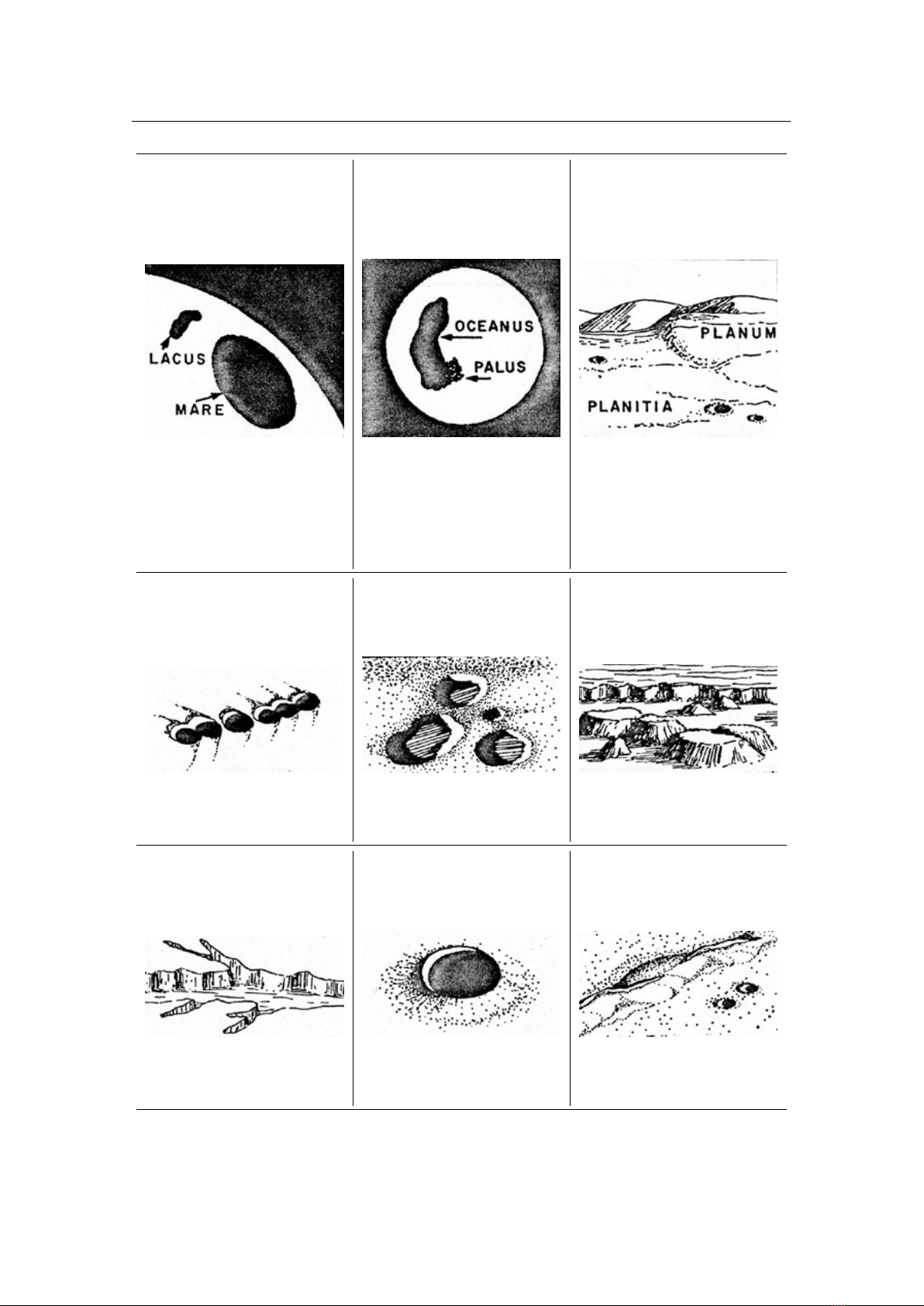
G.4 COPYING IN QUANTITY 407
exchange for copies. If you distribute a large enough number of copies you must also follow the
conditions in section 3.
You may also lend copies, under the same conditions stated above, and you may publicly
display copies.
G.4 COPYING IN QUANTITY
If you publish printed copies (or copies in media that commonly have printed covers) of the
Document, numbering more than 100, and the Document’s license notice requires Cover Texts, you
must enclose the copies in covers that carry, clearly and legibly, all these Cover Texts: Front-Cover
Texts on the front cover, and Back-Cover Texts on the back cover. Both covers must also clearly
and legibly identify you as the publisher of these copies. The front cover must present the full title
with all words of the title equally prominent and visible. You may add other material on the covers
in addition. Copying with changes limited to the covers, as long as they preserve the title of the
Document and satisfy these conditions, can be treated as verbatim copying in other respects.
If the required texts for either cover are too voluminous to fit legibly, you should put the first
ones listed (as many as fit reasonably) on the actual cover, and continue the rest onto adjacent
pages.
If you publish or distribute Opaque copies of the Document numbering more than 100, you must
either include a machine-readable Transparent copy along with each Opaque copy, or state in or
with each Opaque copy a computer-network location from which the general network-using public
has access to download using public-standard network protocols a complete Transparent copy of
the Document, free of added material. If you use the latter option, you must take reasonably prudent
steps, when you begin distribution of Opaque copies in quantity, to ensure that this Transparent
copy will remain thus accessible at the stated location until at least one year after the last time you
distribute an Opaque copy (directly or through your agents or retailers) of that edition to the public.
It is requested, but not required, that you contact the authors of the Document well before
redistributing any large number of copies, to give them a chance to provide you with an updated
version of the Document.
G.5 MODIFICATIONS
You may copy and distribute a Modified Version of the Document under the conditions of sections
2 and 3 above, provided that you release the Modified Version under precisely this License, with
the Modified Version filling the role of the Document, thus licensing distribution and modification
of the Modified Version to whoever possesses a copy of it. In addition, you must do these things in
the Modified Version:
•
A. Use in the Title Page (and on the covers, if any) a title distinct from that of the Document,
and from those of previous versions (which should, if there were any, be listed in the History
section of the Document). You may use the same title as a previous version if the original
publisher of that version gives permission.
•
B. List on the Title Page, as authors, one or more persons or entities responsible for authorship
of the modifications in the Modified Version, together with at least five of the principal authors
of the Document (all of its principal authors, if it has fewer than five), unless they release
you from this requirement.
•
C. State on the Title page the name of the publisher of the Modified Version, as the publisher.
•
D. Preserve all the copyright notices of the Document.
•
E. Add an appropriate copyright notice for your modifications adjacent to the other copyright
notices.
•
F. Include, immediately after the copyright notices, a license notice giving the public permis-
sion to use the Modified Version under the terms of this License, in the form shown in the
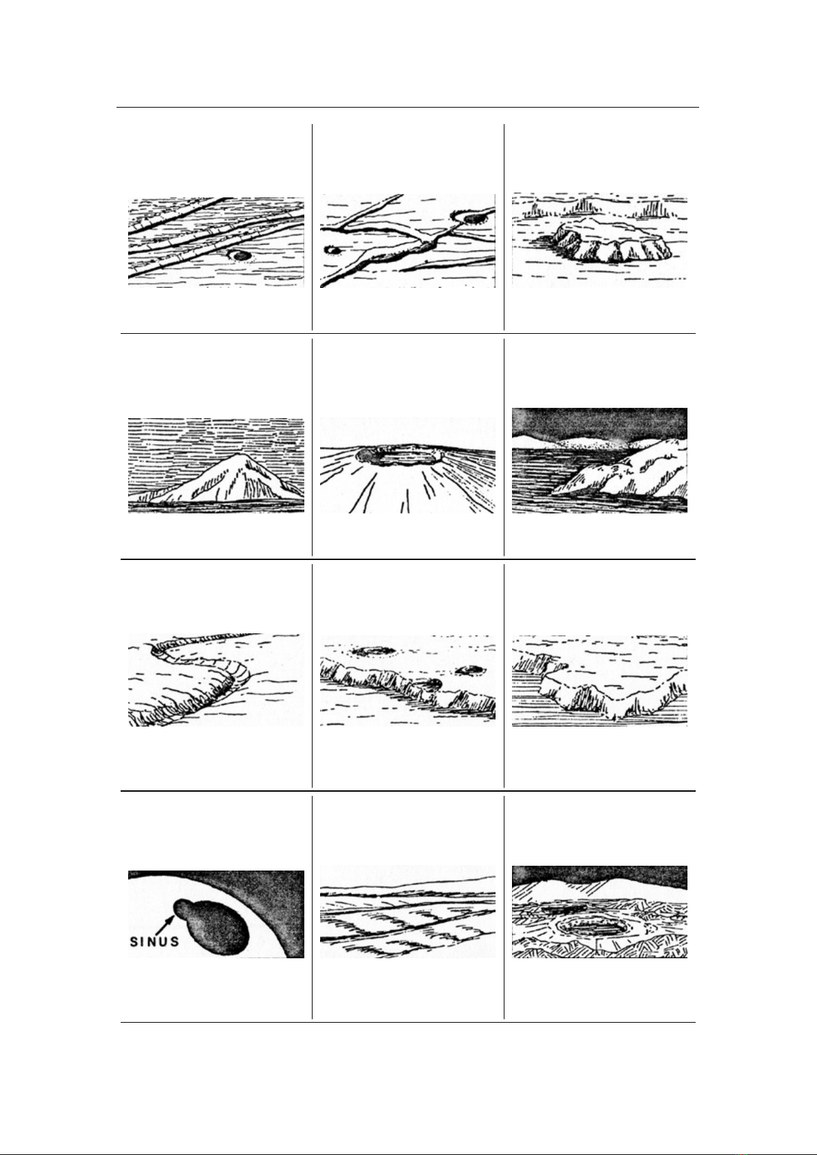
408 Appendix G. GNU Free Documentation License
Addendum below.
•
G. Preserve in that license notice the full lists of Invariant Sections and required Cover Texts
given in the Document’s license notice.
•
H. Include an unaltered copy of this License.
•
I. Preserve the section Entitled “History”, Preserve its Title, and add to it an item stating at
least the title, year, new authors, and publisher of the Modified Version as given on the Title
Page. If there is no section Entitled “History” in the Document, create one stating the title,
year, authors, and publisher of the Document as given on its Title Page, then add an item
describing the Modified Version as stated in the previous sentence.
•
J. Preserve the network location, if any, given in the Document for public access to a
Transparent copy of the Document, and likewise the network locations given in the Document
for previous versions it was based on. These may be placed in the “History” section. You
may omit a network location for a work that was published at least four years before the
Document itself, or if the original publisher of the version it refers to gives permission.
•
K. For any section Entitled “Acknowledgements” or “Dedications”, Preserve the Title of
the section, and preserve in the section all the substance and tone of each of the contributor
acknowledgements and/or dedications given therein.
•
L. Preserve all the Invariant Sections of the Document, unaltered in their text and in their
titles. Section numbers or the equivalent are not considered part of the section titles.
•
M. Delete any section Entitled “Endorsements”. Such a section may not be included in the
Modified Version.
•
N. Do not retitle any existing section to be Entitled “Endorsements” or to conflict in title
with any Invariant Section.
•
O. Preserve any Warranty Disclaimers.
If the Modified Version includes new front-matter sections or appendices that qualify as
Secondary Sections and contain no material copied from the Document, you may at your option
designate some or all of these sections as invariant. To do this, add their titles to the list of Invariant
Sections in the Modified Version’s license notice. These titles must be distinct from any other
section titles.
You may add a section Entitled “Endorsements”, provided it contains nothing but endorsements
of your Modified Version by various parties — for example, statements of peer review or that the
text has been approved by an organization as the authoritative definition of a standard.
You may add a passage of up to five words as a Front-Cover Text, and a passage of up to
25 words as a Back-Cover Text, to the end of the list of Cover Texts in the Modified Version.
Only one passage of Front-Cover Text and one of Back-Cover Text may be added by (or through
arrangements made by) any one entity. If the Document already includes a cover text for the same
cover, previously added by you or by arrangement made by the same entity you are acting on behalf
of, you may not add another; but you may replace the old one, on explicit permission from the
previous publisher that added the old one.
The author(s) and publisher(s) of the Document do not by this License give permission to use
their names for publicity for or to assert or imply endorsement of any Modified Version.
G.6 COMBINING DOCUMENTS
You may combine the Document with other documents released under this License, under the terms
defined in section 4 above for modified versions, provided that you include in the combination all
of the Invariant Sections of all of the original documents, unmodified, and list them all as Invariant
Sections of your combined work in its license notice, and that you preserve all their Warranty
Disclaimers.
The combined work need only contain one copy of this License, and multiple identical Invariant
Sections may be replaced with a single copy. If there are multiple Invariant Sections with the same

G.7 COLLECTIONS OF DOCUMENTS 409
name but different contents, make the title of each such section unique by adding at the end of
it, in parentheses, the name of the original author or publisher of that section if known, or else a
unique number. Make the same adjustment to the section titles in the list of Invariant Sections in
the license notice of the combined work.
In the combination, you must combine any sections Entitled “History” in the various original
documents, forming one section Entitled “History”; likewise combine any sections Entitled “Ac-
knowledgements”, and any sections Entitled “Dedications”. You must delete all sections Entitled
“Endorsements”.
G.7 COLLECTIONS OF DOCUMENTS
You may make a collection consisting of the Document and other documents released under this
License, and replace the individual copies of this License in the various documents with a single
copy that is included in the collection, provided that you follow the rules of this License for verbatim
copying of each of the documents in all other respects.
You may extract a single document from such a collection, and distribute it individually under
this License, provided you insert a copy of this License into the extracted document, and follow
this License in all other respects regarding verbatim copying of that document.
G.8 AGGREGATION WITH INDEPENDENT WORKS
A compilation of the Document or its derivatives with other separate and independent documents
or works, in or on a volume of a storage or distribution medium, is called an “aggregate” if the
copyright resulting from the compilation is not used to limit the legal rights of the compilation’s
users beyond what the individual works permit. When the Document is included in an aggregate,
this License does not apply to the other works in the aggregate which are not themselves derivative
works of the Document.
If the Cover Text requirement of section 3 is applicable to these copies of the Document, then if
the Document is less than one half of the entire aggregate, the Document’s Cover Texts may be
placed on covers that bracket the Document within the aggregate, or the electronic equivalent of
covers if the Document is in electronic form. Otherwise they must appear on printed covers that
bracket the whole aggregate.
G.9 TRANSLATION
Translation is considered a kind of modification, so you may distribute translations of the Document
under the terms of section 4. Replacing Invariant Sections with translations requires special permis-
sion from their copyright holders, but you may include translations of some or all Invariant Sections
in addition to the original versions of these Invariant Sections. You may include a translation of
this License, and all the license notices in the Document, and any Warranty Disclaimers, provided
that you also include the original English version of this License and the original versions of those
notices and disclaimers. In case of a disagreement between the translation and the original version
of this License or a notice or disclaimer, the original version will prevail.
If a section in the Document is Entitled “Acknowledgements”, “Dedications”, or “History”, the
requirement (section 4) to Preserve its Title (section 1) will typically require changing the actual
title.
G.10 TERMINATION
You may not copy, modify, sublicense, or distribute the Document except as expressly provided
under this License. Any attempt otherwise to copy, modify, sublicense, or distribute it is void, and
will automatically terminate your rights under this License.

410 Appendix G. GNU Free Documentation License
However, if you cease all violation of this License, then your license from a particular copyright
holder is reinstated (a) provisionally, unless and until the copyright holder explicitly and finally
terminates your license, and (b) permanently, if the copyright holder fails to notify you of the
violation by some reasonable means prior to 60 days after the cessation.
Moreover, your license from a particular copyright holder is reinstated permanently if the
copyright holder notifies you of the violation by some reasonable means, this is the first time you
have received notice of violation of this License (for any work) from that copyright holder, and you
cure the violation prior to 30 days after your receipt of the notice.
Termination of your rights under this section does not terminate the licenses of parties who
have received copies or rights from you under this License. If your rights have been terminated and
not permanently reinstated, receipt of a copy of some or all of the same material does not give you
any rights to use it.
G.11 FUTURE REVISIONS OF THIS LICENSE
The Free Software Foundation may publish new, revised versions of the GNU Free Documentation
License from time to time. Such new versions will be similar in spirit to the present version, but
may differ in detail to address new problems or concerns. See
http://www.gnu.org/copyleft/
.
Each version of the License is given a distinguishing version number. If the Document specifies
that a particular numbered version of this License “or any later version” applies to it, you have the
option of following the terms and conditions either of that specified version or of any later version
that has been published (not as a draft) by the Free Software Foundation. If the Document does
not specify a version number of this License, you may choose any version ever published (not as a
draft) by the Free Software Foundation. If the Document specifies that a proxy can decide which
future versions of this License can be used, that proxy’s public statement of acceptance of a version
permanently authorizes you to choose that version for the Document.
G.12 RELICENSING
“Massive Multiauthor Collaboration Site” (or “MMC Site”) means any World Wide Web server
that publishes copyrightable works and also provides prominent facilities for anybody to edit
those works. A public wiki that anybody can edit is an example of such a server. A “Massive
Multiauthor Collaboration” (or “MMC”) contained in the site means any set of copyrightable works
thus published on the MMC site.
“CC-BY-SA” means the Creative Commons Attribution-Share Alike 3.0 license published by
Creative Commons Corporation, a not-for-profit corporation with a principal place of business in
San Francisco, California, as well as future copyleft versions of that license published by that same
organization.
“Incorporate” means to publish or republish a Document, in whole or in part, as part of another
Document.
An MMC is “eligible for relicensing” if it is licensed under this License, and if all works
that were first published under this License somewhere other than this MMC, and subsequently
incorporated in whole or in part into the MMC, (1) had no cover texts or invariant sections, and (2)
were thus incorporated prior to November 1, 2008.
The operator of an MMC Site may republish an MMC contained in the site under CC-BY-SA
on the same site at any time before August 1, 2009, provided the MMC is eligible for relicensing.
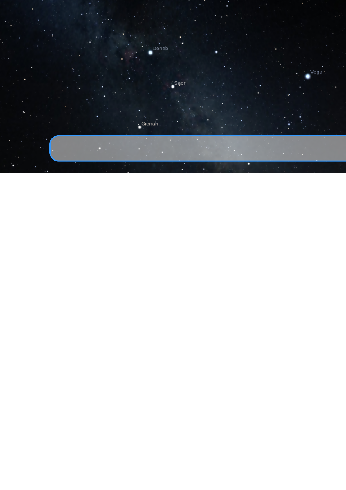
H. Acknowledgements
H.1 Contributors to this User Guide
When not listed as chapter authors, the following were the main contributors to the User Guide, mostly for
versions before V0.15:
Matthew Gates
Primary author of the first User Guide (versions 0.9 to 0.12)
Paul Robinson Sky guide; exercise ideas
Andras Mohari
Celestial sphere diagrams; numerous corrections
Rudy Gobits, Dirk Schwarzhans
Mac platform specifics
Barry Gerdes (†2014)
Windows platform specifics
Customisation of .fab files
Documentation Maintainer up to V0.12
Sigma
Japanese translation; many corrections
Richard Powell
Figure 19.3 (colour/magnitude diagram) is a modification
of his diagram; he kindly granted permission for it to be
distributed under the FDL
John Twin
Many spelling corrections
Georg Zotti Lead author of the 0.15+ editions
Alexander Wolf
New layout, many contributions for the 0.15+ editions
The rest of the Stellarium developer team
You know who you are. . . :-)
Additional material has been incorporated into the guide from sources that are published under the GNU
FDL, including material from Wikipedia and the Astronomy book at Wikibooks.
H.2 Developers
Stellarium is not a company. It is a project created by a community of amateur and professional astronomers,
software engineers, 3D graphics experts, cultural astronomers and experts in other related fields. Together
we created something unique.
H.2.1 Developers
Project coordinator & lead developer Fabien Chéreau
Graphic/other designer Martín Bernardi
Developer Guillaume Chéreau
Developer Georg Zotti
Developer Alexander V. Wolf
Developer Ruslan Kabatsayev
Developer Worachate Boonplod
Developer Henry Leung

412 Appendix H. Acknowledgements
Sky cultures researcher Susanne M. Hoffmann
Tester Khalid AlAjaji
H.2.2 Former Developers
Several people have made significant contributions, but are no longer active. Their work has made a big
difference to the project:
Graphic/other designer Johan Meuris
Doc author/developer Matthew Gates
Developer Johannes Gajdosik
Developer Rob Spearman
Developer Bogdan Marinov
Developer Timothy Reaves
Developer Florian Schaukowitsch
Developer András Mohari
Developer Mike Storm
Developer Ferdinand Majerech
Developer Jörg Müller
Developer Marcos Cardinot
OSX Developer Nigel Kerr
OSX Developer Diego Marcos
Continuous Integration Hans Lambermont
H.2.3 Contributors
Many individuals have made contributions to the project and their work has made Stellarium better. Alpha-
betically sorted list of all contributors:
Adam Majer, Adriano Steffler, Alec Clews, Alessandro Siniscalchi, Alex Gamper, Alexander Belopolsky,
Alexander Duytschaever, Alexander Miller, Alexander V. Wolf, Alexandros Kosiaris, Alexey Dokuchaev,
Alexey Sokolov, Allan Johnson, Andras Mohari, Andrei Borza, Andrew Jeddeloh, Andy Kirkham, Angelo
Fraietta, Annette S. Lee, Antoine Jacoutot, Anton Samoylov, Arjen de Korte, Aspere, Atque, Barry Gerdes,
Bernd K, Björn Höfling, Bogdan Marinov, Brian Kloppenborg, Cassy, Chi Huynh, ChrUnger, Chris Xiao,
Clement Sommelet, Clepalitto, Colin Gaudion, Cosimo Cecchi, Dan Joplin, Dan Smale, Daniel, Daniel
Adastra, Daniel De Mickey, Daniel Michalik, Danny Milosavljevic, Dark Dragon, David Baucum, Dempsey-
p, Dhia, Diego Marcos, Dominik Maximilián Ramík, Edgar Scholz, Elaina, Eleni Maria Stea, Emmanuel,
EuklidAlexandria, Fabien Chereau, Felix Z, Ferdinand Majerech, Florian Schaukowitsch, François Scholder,
Freeman Li, FreewareTips, Froenchenko Leonid, Fòram na Gàidhlig, Georg Zotti, Gion Kunz, GitHaarek,
Giuseppe Putzolu, Greg Alexander, Guillaume Chereau, Guillaume Communie, Gábor Péterffy, Hans
Lambermont, Hector Quemada, Henry Leung, Hernan Martinez, Hleb Valoshka, Holger, Holger Nießner,
Iceflower, Ivan Marti-Vidal, J.L.Canales, JAY RESPLER, JMejuto, Jack Schmidt, Jean-Philippe Lambert,
Jocelyn GIROD, Johan Meuris, Johannes Gajdosik, Jonas Persson, Jörg Müller, Katrin Leinweber, Kenan
Derviševi
´
c, Khalid AlAjaji, Kirill Snezhko, Konrad Rybka, Kutaibaa Akraa, Louis Strous, M.S. Adityan,
Maciej Serylak, Marc Espie, Marcos Cardinot, Martin Bernardi, Martin Bernardi (Laptop), Matt Hughes,
Matthew Gates, Matthias Drochner, Matwey V. Kornilov, Max Digruber, Michael Dickens, Michael Storm,
Michael Taylor, Michal Sojka, Mike Boyle, Mike Garrahan, Minmin Gong, Mircea Lite, Miroslav Broz,
Mykyta Sytyi, Nick Fedoseev, Nick Kanel, Nicolas Martignoni, Nidroide, Nir Lichtman, Norman Rasmussen,
Oleg Ginzburg, Oscar Roig Felius, Paolo Cancedda (Pac), Paolo Stivanin, ParkSangJun, Patrick, Paul Krizak,
Pavel Klimenko, Pawel Stolowski, Peter, Peter Hickey, Peter Mousley, Peter Neubauer, Peter Vasey, Peter
Walser, Petr Kubánek, Pino Toscano, Pluton Helleformer, Qam1, RVS, Ralph Schäfermeier, Ray, Rob
Spearman, Robert S. Fuller, Roland Bosa, Ross Mitchell, Rumen Bogdanovski, Ruslan Kabatsayev, Sam
Lanning, Sebastian Jennen, Sergej Krivonos, Sergey, Shantanu Agarwal, Sibi Antony, SilverAstro, Simon
Parzer, Song Li, Sripath Roy Koganti, Steven Bellavia, Sun Shuwei, Susanne M Hoffmann, Sveinn í Felli,
Tanmoy Saha, Teemu Nätkinniemi, Teresa Huertas, Thilo, Thomas1664, Tig la Pomme, Timothy Reaves,
Tomasz Buchert, Tony Furr, TotalCaesar659, Tuomas Teipainen, T
¯
evita O. Ka
‘
ili, Vancho Stojkoski, Vicente
Reyes, Victor Reijs, Vishvas Vasuki, Vladislav Bataron, Volker Hören, Wang Siliang, William Formyduval,
Wolfgang Laun, Wonkyo Choe, Worachate Boonplod, Yaakov Selkowitz, Youssif Ghantous Filho, Yuri
Chornoivan, Yury Solomonov, adalava, afontenot, bkuhls, bv6679, chithihuynh, colossatr0n, henrysky,
leonardcj, luz paz, luzpaz, misibacsi, pkrawczun, rikardfalkeborn, riodoro1, sebagr, tofilwiktor, uwes-ufo,
ysjbserver, zhu1995zpb, Łukasz ’sil2100’ Zemczak.
H.3 How you can help 413
H.3 How you can help
We especially welcome contributions in shape of working program code for interesting features, but also bug
reports, feature requests and other feedback through the usual channels (trackers, forums and so on):
Stellarium on Github https://github.com/Stellarium/
Questions for Stellarium (FAQ) https://github.com/Stellarium/stellarium/wiki/FAQ
Current issues (FAQ) https://github.com/Stellarium/stellarium/wi ki /Common-Pro bl em
s-for-the-current-version
Google Group https://groups.google.com/group/stellarium
Another form of support, donations, can be given via
https://opencollective.com/stellarium/
donate.
H.4 Technical Articles
Stellarium would not look the same and work without these works from computer graphics and astronomy.
The tone reproductor class
The class mainly performs a fast implementation of the algorithm from Tum-
blin and Rushmeier (1993), with more accurate values from Devlin et al. (2002). The blue shift
formula is taken from Jensen et al. (2000) and combined with the Scotopic vision formula from
Larson, Rushmeier, and Piatko (1997).
The skylight class
The class governs sky colors and is a fast implementation of the algorithm by Preetham,
Shirley, and Smits (1999).
The skybright class
The class governs physical sky brightness values based on Bradley Schaefer’s VIS-
LIMIT.BAS basic source code (B. Schaefer, 1998). The basic sources are available on the Sky and
Telescope web site (code “offered as-is and without support”).
The ∆T calculations For implementation of calculation routines for ∆T we used the following sources:
1. ∆T
webpage by Rob van Gent:
https://webspace.science.uu.nl/~gent0113/deltat
/deltat.htm
2.
Five Millennium Canon of Solar Eclipses: -1900 to +3000 (Espenak and Meeus, 2006) (
https:
//eclipse.gsfc.nasa.gov/SEhelp/deltatpoly2004.html)
3.
Thousand Year Canon of Solar Eclipses 1501 to 2500 (Espenak, 2014) (
https://eclipsew
ise.com/help/deltatpoly2014.html)
4. “On the system of astronomical constants” (Clemence, 1948)
5.
“The rotation of the earth, and the secular accelerations of the sun, moon and planets” (Spencer
Jones, 1939)
6.
“Polynomial approximations for the correction delta T E.T.-U.T. in the period 1800-1975”
(Schmadel and Zech, 1979)
7. “ELP 2000-85 and the dynamic time-universal time relation” (Borkowski, 1988)
8.
“Empirical Transformations from U.T. to E.T. for the Period 1800-1988” (Schmadel and Zech,
1988)
9.
“Historical values of the Earth’s clock error
∆
T and the calculation of eclipses” (Morrison and
F. R. Stephenson, 2004) with Addendum (Morrison and F. R. Stephenson, 2005)
10. “Polynomial approximations to Delta T, 1620-2000 AD” (Meeus and Simons, 2000)
11. Canon of Solar Eclipses -2003 to +2526 (Mucke and Meeus, 1983)
12.
“The accelerations of the earth and moon from early astronomical observations” (Muller and
F. R. Stephenson, 1975)
13. “Pre-Telescopic Astronomical Observations” (F. R. Stephenson, 1978)
14.
“Long-term changes in the rotation of the earth - 700 B.C. to A.D. 1980” (F. R. Stephenson and
Morrison, 1984)
15.
“Long-Term Fluctuations in the Earth’s Rotation: 700 BC to AD 1990” (F. R. Stephenson and
Morrison, 1995)
16. Historical Eclipses and Earth’s Rotation (F. Richard Stephenson, 1997)
17. Astronomical Algorithms (Meeus, 1998)
18. Astronomy on the Personal Computer (Montenbruck and Pfleger, 2000)
19. Calendrical Calculations (The Millennium Edition) (Reingold and Dershowitz, 2001)
20. ∆T webpage by V. Reijs: http://www.iol.ie/~geniet/eng/DeltaTeval.htm
Precession:
“New precession expressions, valid for long time intervals” (Vondrák, Capitaine, and Wallace,
2011) with correction (Vondrák, Capitaine, and Wallace, 2012)
414 Appendix H. Acknowledgements
Nutation:
“An abridged model of the precession-nutation of the celestial pole” (McCarthy and Luzum,
2003) This model provides accuracy better than 1 milli-arcsecond in the time 1995-2050. It is applied
for years -4000..+8000 only.
Martian polar caps: Based on data from Smith et al. (2009) and Piqueux et al. (2015).
Solar limb darkening: Livingston (2002).v 23.1
Color of Neptune: Irwin et al. (2024).v 25.1
H.5 Included Source Code
•
Some computation of the sidereal time (
sidereal_time.h/c
) and Pluto orbit contains code from
the libnova library (LGPL) by Liam Girdwood.
•
The
orbit.cpp/h
and
solve.h
files were directly borrowed from Celestia (Chris Laurel; GPL
license). They have now evolved a bit.
•
Several implementations of IMCCE theories for planet and satellite movement by Johannes Gajdosik
(MIT-style license, see the corresponding files for the license text)
•
The tesselation algorithms were originally extracted from the glues library version 1.4 by Mike
Gorchak <mike@malva.ua> (SGI FREE SOFTWARE LICENSE B).
•
OBJ loader in the Scenery3D plugin based on glObjViewer (c) 2007 dhpoware
•
Parts of the code to work with DE430/DE431 and DE440/DE441 data files have been taken from
Project Pluto (GPL license).
•
The
SpoutLibrary.dll
and header from the SpoutSDK version 2.005 available at
http://spout.
zeal.co (BSD license).
H.6 Data
1.
The Hipparcos star catalog From ESA (European Space Agency) and the Hipparcos mission. ref.
ESA, 1997, The Hipparcos and Tycho Catalogues, ESA SP-1200
http://cdsweb.u-strasbg.fr/
ftp/cats/I/239
2. The solar system data mainly comes from IMCCE and partly from Celestia.
3. Polynesian constellations are based on diagrams from the Polynesian Voyaging Society
4. Chinese constellations are based on diagrams from the Hong Kong Space Museum
5.
Egyptian constellations are based on the work of Juan Antonio Belmonte, Instituto de Astrofisica de
Canarias
6.
The Tycho-2 Catalogue of the 2.5 Million Brightest Stars Hog E., Fabricius C., Makarov V.V., Urban
S., Corbin T., Wycoff G., Bastian U., Schwekendiek P., Wicenec A. Astron. Astrophys. 355, L27
(2000) http://cdsweb.u-strasbg.fr/ftp/cats/I/259
7.
Naval Observatory Merged Astrometric Dataset (NOMAD) version 1 (
http://www.nofs.navy.mi
l/nomad) Norbert Zacharias writes:
“There are no fees, both UCAC and NOMAD are freely available with the only
requirement that the source of the data (U.S. Naval Observatory) and original product
name need to be provided with any distribution, as well as a description about any changes
made to the data, if at all.”
The changes made to the data are:
•
try to compute visual magnitude and color from the b,v,r values
•
compute nr_of_measurements = the number of valid b, v, r values
•
throw away or keep stars (depending on magnitude, nr_of_measurements, combination of flags,
tycho2 number)
•
add all stars from Hipparcos (incl. component solutions), and tycho2+1st supplement
•
reorganize the stars in several brightness levels and triangular zones according to position and
magnitude
The programs that are used to generate the star files are called MakeCombinedCatalogue, ParseHip,
ParseNomad, and can be found in the util subdirectory in source code. The position, magnitudes,
and proper motions of the stars coming from NOMAD are unchanged, except for a possible loss
of precision, especially in magnitude. When there is no V magnitude, it is estimated from R or B
magnitude. When there is no B or V magnitude, the color B-V is estimated from the other magnitudes.
Also proper motions of faint stars are neglected at all.
H.7 Graphics 415
8.
Stellarium’s Catalog of Variable Stars based on General Catalog of Variable Stars (GCVS) version
2013Apr.
http://www.sai.msu.su/gcvs/gcvs/
Samus N.N., Durlevich O.V., Kazarovets E V.,
Kireeva N.N., Pastukhova E.N., Zharova A.V., et al., General Catalogue of Variable Stars (Samus+
2007-2012) http://cdsarc.u-strasbg.fr/viz-bin/Cat?cat=B%2Fgcvs&
9. Consolidated DSO catalog was created from various data:
a. NGC/IC data taken from SIMBAD Astronomical Database http://simbad.u-strasbg.fr
b.
Distance to NGC/IC data taken from NED (NASA/IPAC EXTRAGALACTIC DATABASE)
http://ned.ipac.caltech.edu
c.
Catalogue of HII Regions (Sharpless, 1959) (
http://vizier.u-strasbg.fr/viz-bin/V
izieR?-source=VII/20)
d.
H-
α
emission regions in the Southern Milky Way (Rodgers+, 1960) (
http://vizier.u-str
asbg.fr/viz-bin/VizieR?-source=VII/216)
e.
Catalogue of Reflection Nebulae (Van den Bergh, 1966) (
http://vizier.u-strasbg.fr/
viz-bin/VizieR?-source=VII/21)
f.
Lynds’ Catalogue of Dark Nebulae (LDN) (Lynds, 1962) (
http://vizier.u-strasbg.fr/
viz-bin/VizieR?-source=VII/7A)
g.
Lynds’ Catalogue of Bright Nebulae (Lynds, 1965) (
http://vizier.u-strasbg.fr/viz-b
in/VizieR?-source=VII/9)
h.
Catalog of bright diffuse Galactic nebulae (Cederblad, 1946) (
http://vizier.u-strasbg.f
r/viz-bin/VizieR?-source=VII/231)
i.
Barnard’s Catalogue of 349 Dark Objects in the Sky (Barnard, 1927) (
http://vizier.u-str
asbg.fr/viz-bin/VizieR?-source=VII/220A)
j.
A Catalogue of Star Clusters shown on Franklin-Adams Chart Plates (Melotte, 1915) from
NASA ADS (http://adsabs.harvard.edu/abs/1915MmRAS..60..175M)
k.
On Structural Properties of Open Galactic Clusters and their Spatial Distribution. Catalog of
Open Galactic Clusters (Collinder, 1931) from NASA ADS (
http://adsabs.harvard.edu
/abs/1931AnLun...2....1C)
l.
The Collinder Catalog of Open Star Clusters. An Observer’s Checklist. Edited by Thomas
Watson from CloudyNights (
http://www.cloudynights.com/page/articles/cat/art
icles/the-collinder-catalog-updated-r2467)
10. Cross-identification of objects in consolidated DSO catalog was made with:
a. SIMBAD Astronomical Database http://simbad.u-strasbg.fr
b.
Merged catalogue of reflection nebulae (Magakian, 2003)
http://vizier.u-strasbg.fr/
viz-bin/VizieR-3?-source=J/A+A/399/141
c.
Messier Catalogue from Wikipedia (includes morphological classification and distances)
https:
//en.wikipedia.org/wiki/List_of_Messier_objects
d.
Caldwell Catalogue from Wikipedia (includes morphological classification and distances)
https://en.wikipedia.org/wiki/Caldwell_catalogue
11.
Morphological classification and magnitudes (partially) for Melotte catalogue from DeepSkyPedia
http://deepskypedia.com/wiki/List:Melotte
H.7 Graphics
All graphics are copyrighted by the Stellarium’s Team (GNU GPLv2 or later) except the ones mentioned
below:
•
The “earthmap” texture was created by NASA (Reto Stockli, NASA Earth Observatory) using data
from the MODIS instrument aboard the Terra satellite (Public Domain). See section H.7.1 for full
credits.
•
Moon texture map was combined from maps by USGS Astrogeology Research Program,
http:
//a strogeol ogy.usgs.gov
(Public Domain, DFSG-free) and by Lunar surface textures from
Celestia, based on Clementine data (Public Domain).
•
Jupiter map created by James Hastings-Trew from Cassini data. “The maps are free to download and
use as source material or resource in artwork or rendering (CGI or real time).”
•
The Sun and Iapetus maps, and rings of Uranus are from Celestia (
http://shatters.net/celes
tia/) under the GNU General Purpose License, version 2 or any later version:
– Iapetus map is from dr. Fridger Schrempp (t00fri).
•
The Amalthea, Europa, Ganymede, Gaspra,Mercury, Uranus, Neptune, Mimas, Bianca, Epimetheus,
416 Appendix H. Acknowledgements
Ida, Vesta, Hyperion, Io, Janus, Phoebe, Saturn, Tethys, Venus, Ceres, Uranus, Epimetheus, Deimos,
Proteus and comet maps are processed by Oleg Pluton a.k.a Helleformer License: Creative Commons
Attribution 4.0 International
•
The Titania, Umbriel, Pluto, Charon, Sedna and 2007 OR10 maps are created by Kexitt and postpro-
cessed by Oleg Pluton a.k.a Helleformer License: Creative Commons Attribution 4.0 International
•
The Ariel, Haumea, Miranda, Oberon and Nereid maps are created by Snowfall and postprocessed by
Oleg Pluton a.k.a Helleformer License: Creative Commons Attribution 4.0 International
•
The Eris and Dysnomia maps are created by MrSpace43 and postprocessed by Oleg Pluton a.k.a
Helleformer License: Creative Commons Attribution 4.0 International
•
The Rhea map are created by FarGetaNik and postprocessed by Oleg Pluton a.k.a Helleformer License:
Creative Commons Attribution 4.0 International
•
The Titan (Clouds) map are created by Magenta Meteorite and postprocessed by Oleg Pluton a.k.a
Helleformer License: Creative Commons Attribution 4.0 International
•
Callisto map is created by John van Vliet from PDS data and modified by RVS. License: cc-by-sa.
•
Dione and Enceladus maps are created by NASA (CICLOPS team) from Cassini data, colored by
RVS. Public domain.
•
All other planet maps from David Seal’s site:
http://maps.jpl.nasa.gov/
see license in section
H.7.2
•
Bennu map is created by NASA from OSIRIS-REx spacecraft data. Public domain. Full size mosaic:
https://www.asteroidmission.org/bennu_global_mosaic/
•
The fullsky milky way panorama is created by Axel Mellinger, University of Potsdam, Germany.
Further information and more pictures available from
http://home.arcor-online.de/axel.me
llinger/
License: permission given to “Modify and redistribute this image if proper credit to the
original image is given.”
•
All messiers nebula pictures except those mentioned below from the Grasslands Observatory : “Images
courtesy of Tim Hunter and James McGaha, Grasslands Observatory at
http://www.3towers.com
.”
License: permission given to “use the image freely” (including right to modify and redistribute) “as
long as it is credited.”
•
M31 pictures come from LEE ang HG731GZ License: Creative Commons Attribution 3.0 Unported
•
Images of NGC4526, NGC6544, NGC6553 from Yang Kai License: public domain
•
Images of M1, M27, M57, M97, NGC6946 from Stephane Dumont
•
Images of NGC856, NGC884 from Maxime Spano
•
Constellation art, GUI buttons, logo created by Johan Meuris (jomejome at users.sourceforge.net)
http://www.joh anmeuris.eu/
License: released under the Free Art License (
http://artlib
re.org/ licence.php/lalgb.html
) Icon created by Johan Meuris License: Creative Commons
Attribution-ShareAlike 3.0 Unported
•
The “earth-clouds” texture includes imagery owned by NASA. See NASA’s Visible Earth project at
http://visibleearth.nasa.gov/ License:
1. The imagery is free of licensing fees
2. NASA requires that they be provided a credit as the owners of the imagery
The cloud texturing was taken from Celestia (GPL), http://www.shatters.net/celestia/
•
The folder icon derived from the Tango Desktop Project, used under the terms of the Creative
Commons Attribution Share-Alike license.
•
Images of NGC7317, NGC7319, NGC7320 from Andrey Kuznetsov, Kepler Observatory
http:
//kepler-observatorium.ru License: Creative Commons Attribution 3.0 Unported
•
Images of NGC2903, NGC3185, NGC3187, NGC3189, NGC3190, NGC3193, NGC3718, NGC3729,
NGC5981, NGC5982, NGC5985 from Oleg Bryzgalov
http://olegbr. astroclub.kiev.ua/
License: Creative Commons Attribution 3.0 Unported
•
Image of eta Carinae from Harel Boren
http://www.pbase.com/
License: Creative Commons
Attribution-Share Alike 4.0 International
•
Images of NGC3726 from KPNO/NOIRLab/NSF/AURA/George Hickey/Adam Block, post-processing:
Sun Shuwei
https://noirlab.edu/public/
License: Creative Commons Attribution 4.0 Interna-
tional
•
Images of M21, M47, NGC3324, NGC7590, RCW158 from Trevor Gerdes
http://www.sarcasmo
gerdes.com/
•
Images of NGC1532 from users of Ice In Space http://www.iceinspace.com.au/
•
Images of NGC3293 from ESO/G. Beccari
http://eso.org/public/
License: Creative Commons
H.7 Graphics 417
Attribution 4.0 International
•
Images of SMC (Magellanic Clouds) from Albert Van Donkelaar
•
Images of NGC1261, NGC3201, NGC4833, NGC5286, NGC5823, NGC6025, NGC6087, NGC6101,
NGC6124, NGC6352, NGC6397, NGC6541, NGC6752 from Tian Mai, Image processing: Sun
Shuwei License: Creative Commons Attribution 4.0 International
•
The Vesta and Ceres map was taken from USGS website
https://astrogeology.usgs.gov/
and
colored by RVS. License: public domain.
•
Images of M15, M24, M51, M58, M63, M76, M82, M96, M101, M105, M106, IC1727, NGC246,
NGC457, NGC467, NGC470, NGC474, NGC488, NGC672, NGC691, NGC1514, NGC1961,
NGC2174, NGC2371, NGC2392, NGC2403, NGC2506, NGC2655, NGC2685, NGC2805, NGC2814,
NGC2820, NGC2841, NGC3079, NGC3166, NGC3310, NGC3344, NGC3359, NGC3504, NGC3512,
NGC3521, NGC3938, NGC4151, NGC4274, NGC4535, NGC4559, NGC4631, NGC4656, NGC4657,
NGC5033, NGC5363, NGC7008, NGC7331, NGC7479, NGC7640, NGC7789, PGC1803573,
Barnard 142, Barnard 173, Sh2-101, Sh2-188, LDN1235, Sadr region (Gamma Cygni), Medusa,
Jones-Emberson 1, NGC2146 from Peter Vasey, Plover Hill Observatory
http://www.madpc.co.u
k/~peterv/
•
Image of IC3568 from Howard Bond (Space Telescope Science Institute), Robin Ciardullo (Pennsyl-
vania State University) and NASA License: public domain
•
Image of solar corona from eclipse 2008-08-01 by Georg Zotti
•
Images of NGC2359 from Carole Pope
https://sites.google.com/site/caroleastroimagi
ng/
•
Images of NGC2261, NGC2818, NGC2936, NGC3314, NGC3690, NGC3918, NGC4038-4039,
NGC5257, NGC5307, NGC6027, NGC6050, NGC6369, NGC6826, NGC7742, IC883, IC4406,
PGC2248, UGC1810, UGC8335, UGC9618, Red Rectangle and Calabash Nebula from NASA,
ESA, the Hubble Heritage (STScI/AURA)-ESA/Hubble Collaboration License: public domain;
http://hubblesite.org/copyright/
•
Image of NGC40 from Steven Bellavia
•
Images of NGC2467, NGC6590, Barnard Loop, IC342 from Sun Shuwei License: public domain
•
Images of M77, NGC3180, NGC5474, NGC6231, Sh2-264, Sh2-308, LDN1622 from Wang Lingyi
License: public domain
•
Images of PGC6830, PGC29653 from Lowell Observatory
http://www2.lowe ll.edu/
License:
public domain
•
Images of M89, IC2220, IC2631, NGC1433, NGC2434, NGC3572, PGC10074, RCW32, RCW38,
RCW49, Fornax Cluster, Virgo Cluster from ESO/Digitized Sky Survey 2
http://eso.org/publ
ic/ License: Creative Commons Attribution 4.0 International
•
Images of NGC3603 from ESO/La Silla Observatory
http://eso.org/public/
License: Creative
Commons Attribution 4.0 International
•
Images of NGC4228, NGC4244 from Ole Nielsen License: Creative Commons Attribution-Share
Alike 2.5 Generic
•
Images of NGC2808, NGC7023, Hercules Cluster from NASA License: public domain
•
Images of M44, IC1396 from Giuseppe Donatiello License: Creative Commons CC0 1.0 Universal
Public Domain Dedication
•
Images of M12, M14, M20, M22, M55, M56, M62, M88, M92, M108, IC5146, NGC225, NGC281,
NGC663, NGC891, NGC1931, NGC6823, NGC7814 from Hewholooks
https://commons.wiki
media.org/wiki/ License: Creative Commons Attribution-Share Alike 3.0 Unported
•
Images of NGC4565 from Ken Crawford
http://www.imagingdeepsky.com/
License: This work
is free and may be used by anyone for any purpose. If you wish to use this content, you do not need to
request permission as long as you follow any licensing requirements mentioned on this page.
•
Images of M61, M64, M65, M66, M91, M99, M100, NGC613, NGC772, NGC918, NGC1042,
NGC1360, NGC1398, NGC1501, NGC1535, NGC1555, NGC2158, NGC2282, NGC2346, NGC2362,
NGC2440, NGC2683, NGC2775, NGC3132, NGC3242, NGC3486, NGC3750, NGC4170, NGC4216,
NGC4361, NGC4395, NGC4414„NGC4450, NGC4676, NGC4725, NGC5216, NGC5248, NGC5426,
NGC5466, NGC6302, NGC6522, NGC6543, NGC6563, NGC6781, NGC6894, NGC7000, NGC7354,
NGC7822, SH2-136, UGC3697, Abell31, Abell33, Abell39, Cassiopeia A, LBN438, Wild’s Triplet
from Adam Block/Mount Lemmon SkyCenter/University of Arizona
http://www.caelumobserv
atory.com/ License: Creative Commons Attribution-Share Alike 3.0 Unported
•
Images of IC1295, NGC134, NGC92, NGC55, NGC908, NGC936, NGC1232, NGC1313, NGC1792,
418 Appendix H. Acknowledgements
NGC1978, NGC2207, NGC2736, NGC3199, NGC3699, NGC3766, NGC3532, NGC4945, NGC5128,
NGC5189, NGC6537, NGC6769, NGC6822, NGC7793 from ESO
http://eso.org/public/
License: Creative Commons Attribution 4.0 International
•
Images of M33, M42, NGC253, NGC5566, LBN782, the Pleiades from HG731GZ License: Creative
Commons Attribution 3.0 Unported
•
Images of M8, M17, M94, IC2944, IC4628, NGC5367, NGC6357, NGC6334, NGC7293, LDN43,
SMC (Hydrogen Alpha) from Dylan O’Donnell
http://deography.com/
License: public domain
•
Images of NGC247 No machine-readable source provided. Own work assumed (based on copyright
claims). No machine-readable author provided. Fany Toporenko assumed (based on copyright claims).
License: Permission is granted to copy, distribute and/or modify this document under the terms of the
GNU Free Documentation License, Version 1.2 or any later version published by the Free Software
Foundation; with no Invariant Sections, no Front-Cover Texts, and no Back-Cover Texts. A copy of
the license is included in the section entitled GNU Free Documentation License.
•
Images of Sh2-73, Sh2-129 from Maurizio Cabibbo, post-processing: Sun Shuwei
https://common
s.wikimedia.org/wiki/ License: Creative Commons Attribution-Share Alike 4.0 International
•
Images of M16, IC4592, IC4601, NGC4236, NGC6914, Perseus Cluster from Sun Gang License:
Creative Commons Attribution-Share Alike 3.0 Unported
•
Images of NGC4651, NGC5906 from R. Jay GaBany
https://www.cosmotography.co m / i m a g
es/ License: Creative Commons Attribution-Share Alike 3.0 Unported
•
Images of NGC7662 from Gianluca.pollastri
https://commons.wikimedia.org/wiki/
License:
Creative Commons Attribution-Share Alike 4.0 International
•
Images of M2, M3, M4, M5, M13, M10, M28, M30, M53, M69, M71, M75, M85, M102, M107, IC10,
NGC6144, PGC143, UGC12613 from Starhopper
https://commons.wikimed ia.org/wiki/
License: Creative Commons Attribution-Share Alike 4.0 International
•
Images of M95, NGC520, NGC660, NGC925, NGC1300, NGC4490, NGC6888, NGC7129, NGC7497
from Jschulman555
https://commons.wikimedia.org/wiki/
License: Creative Commons At-
tribution 3.0 Unported
•
Images of M98 from Clh288
ht tps://commons.wikimedia. org/wiki/
License: Creative
Commons Attribution-Share Alike 2.5 Generic
•
Images of NGC6818 from Robert Rubin (NASA/ESA Ames Research Center), Reginald Dufour
and Matt Browning (Rice University), Patrick Harrington (University of Maryland), and NASA/ESA
https://www.spacetelescope.org/ License: Creative Commons Attribution 4.0 International
•
Images of NGC6188 from Ivan Bok
https://commons.wikimedia.org/wiki/
License: Creative
Commons Attribution 3.0 Unported
•
Images of NGC6188 from Friendlystar
https://commons.wikimedia. org/wiki/
License:
Creative Commons Attribution 3.0 Unported
•
Images of NGC1023 from Fryns Fryns
https://commons.wikimedia.org/wiki/
License: public
domain
•
Images of NGC1269, NGC3195 from Zhu Ying License: Creative Commons Attribution 3.0 Unported
•
Images of IC2118, NGC1499 from Zhao Jingna License: Creative Commons Attribution 3.0 Unported
•
Images of UGC10822 from Science NASA, ESA, Eduardo Vitral (STScI), Roeland van der Marel
(STScI), Sangmo Tony Sohn (STScI), DSS Image Processing: Joseph DePasquale (STScI)
https:
//noirlab.edu/public/ License: Public domain
•
Images of IC2169, NGC2244, NGC3077, SH2-155, SH2-263, Barnard 22, Barnard207, Abell85
from Keesscherer
https://com mons.wikimedia.org/wiki/
License: Creative Commons
Attribution-Share Alike 4.0 International
•
Images of NGC3115 from Mi Lan License: Creative Commons Attribution 3.0 Unported
•
Images of NGC3621 from ESO and Joe DePasquale
http://eso.org/public/
License: Creative
Commons Attribution 4.0 International
•
Images of NGC2547 from ESO/J.Perez
http://eso.org/public/
License: Creative Commons
Attribution 4.0 International
•
Images of M83 from TRAPPIST/E. Jehin/ESO
http://eso.org/public/
License: Creative
Commons Attribution 4.0 International
•
Images of DWB111, IC405, IC410, IC443, IC1805, IC1848, IC2177, NGC288, NGC404, NGC1097,
NGC1931, NGC2264, LBN437, Sh2-191, Sh2-247 from Giuseppe Donatiello, post-processing: Sun
Shuwei
https://flickr.com/photos/133259498@N05/
License: Creative Commons CC0 1.0
Universal Public Domain Dedication
H.7 Graphics 419
•
Images of NGC1055 from Jeffjnet
http://www.iceinspace.com.au/
License: Creative Com-
mons Attribution-Share Alike 3.0 Unported
•
Images of NGC2867, NGC6884 from Howard Bond (ST ScI) and NASA/ESA
https://www.spac
etelescope.org/ License: Creative Commons Attribution 4.0 International
•
Images of NGC4567 from Klaus Hohmann
https://commons.wikimedia.org/wiki
License:
Creative Commons Attribution-Share Alike 3.0 Germany
•
Images of RCW53 from Kong Fanxi License: Creative Commons Attribution-Share Alike 3.0
Unported
•
Images of NGC5897 from San Esteban
http://www.astrosurf.com
License: Creative Commons
Attribution-Share Alike 3.0 Unported
•
Images of NGC6388 from ESO, F. Ferraro (University of Bologna)
http://eso.org/public/
License: Creative Commons Attribution 4.0 International
•
Images of NGC7380, SH2-80, SH2-106 from Cristina Cellini
https://commons.wikimedia.or
g/wiki/ License: Creative Commons Attribution 4.0 International
•
Images of NGC6744 from Zhuokai Liu, Jiang Yuhang License: Creative Commons Attribution 4.0
International
•
Images of NGC2170, SH2-240 from Rogelio Bernal Andreo
https://commons.wikimedia.org/
wiki/ License: Creative Commons Attribution-Share Alike 3.0 Unported
•
Images of VDB 152 from Hubble Space Telescope
https://commons.wikimedia.org/wiki/
License: Creative Commons Attribution-Share Alike 4.0 International
•
Images of NGC6905 from Tom Wildoner
https://commons.wikimedia.org/ wiki/
License:
Creative Commons Attribution-Share Alike 4.0 International
•
Images of NGC2623 from NASA, ESA and A. Evans (Stony Brook University, New York, University
of Virginia & National Radio Astronomy Observatory, Charlottesville, USA)
https://www.spacet
elescope.org/ License: Creative Commons Attribution 4.0 International
•
Images of IC4634, NGC3808, NGC5882, NGC6210, NGC6572, NGC6741 from ESA/Hubble
& NASA
https://www.spacetelescope.org/
License: Creative Commons Attribution 4.0
International
•
Images of NGC6240, PGC33423 from NASA, ESA, the Hubble Heritage (STScI/AURA)-ESA/Hubble
Collaboration, and A. Evans (University of Virginia, Charlottesville/NRAO/Stony Brook University)
https://www.spacetelescope.org/ License: Creative Commons Attribution 4.0 International
•
Images of UGC5470 from Friendlystar
https://ko.wikipedia.org/
License: Creative Commons
Attribution 3.0 Unported
•
Images of UGC6253, UGC9749 from Giuseppe Donatiello
https://en.wikipedia.org/
License:
public domain
•
Images of UGC10214 from NASA, Holland Ford (JHU), the ACS Science Team and ESA
https:
//www.spacetelescope.org/ License: Creative Commons Attribution 4.0 International
•
Images of NGC6503, NGC7714, Hydra Cluster from NASA, ESA, Digitized Sky Survey 2
https:
//www.spacetelescope.org/ License: Creative Commons Attribution 4.0 International
•
Images of NGC2477 from Guillermo Abramson
https://commons.w iki media.org/wiki/
License: Creative Commons Attribution 3.0 Unported
•
Images of NGC4755 from ESO/Y. Beletsky
http://eso.org/public/
License: Creative Commons
Attribution 4.0 International
•
Images of NGC7538 from J. Aleu
https://commons.wikimedia.org /wiki/
License: public
domain
•
Images of IC2395, IC4756, NGC3114, NGC6633 from Roberto Mura
https://en.wikipedia.o
rg/ License: Creative Commons Attribution-Share Alike 3.0 Unported
•
Images of NGC362 from ESO/VISTA VMC
http://eso.org/public/
License: Creative Com-
mons Attribution 4.0 International
•
Images of NGC2997 from Adam Block/ChileScope
http://www.caelumobservatory.com/
License: Creative Commons Attribution-Share Alike 3.0 Unported
•
Images of M74, NGC1788, NGC5053, Sh2-132, Coma Cluster, Leo Cluster, barnard150, LDN673
from Bart Delsaert
https://delsaert.com/
License: Creative Commons Attribution 3.0 Unported
•
Images of NGC1333 from AAE-Agrupacio Astronomica d’Eivissa
https://commons.wikimedia.
org/wiki/ License: Creative Commons Attribution-Share Alike 4.0 International
•
Images of NGC5139 from Jose Mtanous
https://commons.wikimedia.org/wiki/
License:
Creative Commons Attribution-Share Alike 3.0 Unported

420 Appendix H. Acknowledgements
•
Images of NGC6960 from Jose Mtanous
https://commons.wikimedia.org/wiki/
License:
public domain
•
Images of NGC6445 from The Pan-STARRS1 Surveys (PS1) and the PS1 public science archive
have been made possible through contributions by the Institute for Astronomy, the University of
Hawaii, the Pan-STARRS Project Office, the Max-Planck Society and its participating institutes, the
Max Planck Institute for Astronomy, Heidelberg and the Max Planck Institute for Extraterrestrial
Physics, Garching, The Johns Hopkins University, Durham University, the University of Edinburgh,
the Queen’s University Belfast, the Harvard-Smithsonian Center for Astrophysics, the Las Cumbres
Observatory Global Telescope Network Incorporated, the National Central University of Taiwan, the
Space Telescope Science Institute, the National Aeronautics and Space Administration under Grant
No. NNX08AR22G issued through the Planetary Science Division of the NASA Science Mission
Directorate, the National Science Foundation Grant No. AST-1238877, the University of Maryland,
Eotvos Lorand University (ELTE), the Los Alamos National Laboratory, and the Gordon and Betty
Moore Foundation.
https://ps1images.stsci.edu/cgi-bin/ps1cuto uts
License: public
domain
•
Images of LMC (Magellanic Clouds) from ESO/R. Gendler and Sun Shuwei
http://eso.org/pu
blic/
License: Creative Commons Attribution 4.0 International. This work is a derivative of “Map
of the Large Magellanic Cloud” and “The entire Large Magellanic Cloud with annotations” by ESO/R.
Gendler, used under Creative Commons Attribution 4.0 International. This work is licensed under
Creative Commons Attribution 4.0 International by Sun Shuwei.
•
Images of rho Oph from ESO/S. Guisard
http://eso.org/public/
License: Creative Commons
Attribution 4.0 International
•
Images of IC59, IC63 from Zhang Ruiping License: Creative Commons Attribution 4.0 International
•
Images of NGC6366 from Robert Eder, post-processing: Sun Shuwei
https://commons.wikime
dia.org/wiki/ License: Creative Commons Attribution-Share Alike 4.0 International
•
Images of IC418, IC4593, NGC5315, NGC6751 from NASA/ESA and The Hubble Heritage Team
(STScI/AURA)
https://www.s pacetelescope.org/
License: Creative Commons Attribution
4.0 International
•
Images of NGC7009 from ESO/J. Walsh
http://eso.org/public/
License: Creative Commons
Attribution 4.0 International
•
Images of NGC7027 from Judy Schmidt
https://commons.wikimedia.org/wiki/
License:
public domain
•
Images of NGC6309, NGC6891 from Fabian RRRR
https://commons.wikimedia.org/wiki/
License: Creative Commons Attribution-Share Alike 3.0 Unported
•
Images of NGC2022 from ESA/Hubble & NASA, R. Wade
https://www.spacetelescope.org/
License: Creative Commons Attribution 4.0 International
•
Images of NGC654 from Antonio F. Sanchez
https://commons.wikimedia.org/wiki/
License:
Creative Commons Attribution-Share Alike 4.0 International
•
Images of NGC6496 from Mohamad Abbas
https://commons.wikimedia.org/wiki/
License:
Creative Commons Attribution-Share Alike 3.0 Unported
•
Images of PGC3589 from ESA/Hubble, Digitized Sky Survey 2
https://www.spacetelescope.o
rg/ License: Creative Commons Attribution 4.0 International
•
Images of NGC1672 from Davide De Martin (ESA/Hubble), the ESA/ESO/NASA Photoshop FITS
Liberator & Digitized Sky Survey 2
https://www.spacetelescope.org/
License: Creative
Commons Attribution 4.0 International
•
Images of NGC4298 from NASA, ESA, Digitized Sky Survey 2; Acknowledgement: Davide De
Martin
https://www.space telescope.org/
License: Creative Commons Attribution 4.0
International
•
Images of NGC1502 from Kamil Pecinovsky
https://commons.wikimedia.org/wiki/
License:
Creative Commons Attribution-Share Alike 4.0 International
•
Images of NGC752 from Tayson82
https://commons.wikimedia.org/wiki/
License: Creative
Commons Attribution-Share Alike 4.0 International
•
Images of Sh2-170 from Wang Wei License: Creative Commons Attribution-Share Alike 3.0 Unported
•
Images of NGC2613 from ESO/IDA/Danish 1.5 m/R. Gendler, J.-E. Ovaldsen, C. Thone and C. Feron
http://eso.org/public/ License: Creative Commons Attribution 4.0 International
•
The
miscWorldMap.jpg
image was created from NASA Blue Marble Next Generation dataset for
July 2004. Public domain.
https://visibleearth.nasa.gov/images/74092/july-blue-m
H.7 Graphics 421
arble-next-generation
•
Images of M80, M90, RCW101 from NOIRLab/NSF/AURA, post-processing: Sun Shuwei
https:
//commons.wikimedia.org/wiki/ License: Creative Commons Attribution 4.0 International
•
Images of Dark Doodad Nebula, IC1613, NGC1216, NGC4372 from Hansjorg Walchli, post-
processing: Sun Shuwei
https://www.deepskycorner.ch/index.de.php
License: Creative
Commons Attribution 4.0 International
•
Images of NGC1566, NGC1808 from Dark Energy Survey/DOE/FNAL/DECam/CTIO/NOIRLab/NS-
F/AURA, Image processing: T.A. Rector (University of Alaska Anchorage/NSF NOIRLab), J. Miller
(Gemini Observatory/NSF NOIRLab), M. Zamani & D. de Martin (NSF NOIRLab), post-processing:
Sun Shuwei
https://www.deepskycorner.ch/index.de.php
License: Creative Commons
Attribution 4.0 International
•
Images of IC289, NGC185 from Thedarksideobservatory, post-processing: Sun Shuwei
https:
//comm ons.wikimedia.org/wiki/
License: Creative Commons Attribution-Share Alike 4.0
International
•
Images of NGC5005 from KPNO/NOIRLab/NSF/AURA/Ray and Emily Magnani/Adam Block
http
s://commons.wikimedia.org/wiki/ License: Creative Commons Attribution 4.0 International
•
Images of NGC80, NGC147, NGC1491, NGC1624, NGC7026 from Radek Chromik, post-processing:
Sun Shuwei
https://www.deepskycorner.ch/index.de.php
License: Creative Commons
Attribution 4.0 International
•
Images of IC4954 from KPNO/NOIRLab/NSF/AURA/Adam Block, post-processing: Sun Shuwei
https://noirlab.edu/public/ License: Creative Commons Attribution 4.0 International
•
Images of IC2574, Sh2-313 from Jerry Macon, post-processing: Sun Shuwei
https://commons.wi
kimedia.org/wiki/ License: Creative Commons Attribution 4.0 International
•
Images of NGC5395 from KPNO/NOIRLab/NSF/AURA/Doug Matthews and E. J. Jones/Adam
Block, post-processing: Sun Shuwei
https://commons.wikimedia.org/wiki/
License: Creative
Commons Attribution 4.0 International
•
Images of RCW77 from KPNO/NOIRLab/NSF/AURA/Doug Matthews and E. J. Jones/Adam Block,
post-processing: Sun Shuwei https://esahubble.org/ License: public domain
•
Images of Sh2-216 from Ram samudrala, post-processing: Sun Shuwei
https://commons.wikime
dia.org/wiki/ License: Creative Commons Attribution 4.0 International
•
Images of Sh2-174, Sh2-239 from T.A. Rector (University of Alaska Anchorage) and H. Schweiker
(WIYN and NOIRLab/NSF/AURA), post-processing: Sun Shuwei
https://noirlab.edu/publ
ic/ License: Creative Commons Attribution 4.0 International
•
Images of Sh2-82, Sh2-91, Sh2-119, Sh2-135, Sh2-235, Sh2-261, VDB158 from Sebastian Goralik,
post-processing: Sun Shuwei
https://flickr.com /photos/sebastiangoralik/
License:
Creative Commons CC0 1.0 Universal Public Domain Dedication
•
Images of NGC4976 from ESO/Dss2, Giuseppe Donatiello, post-processing: Sun Shuwei
https:
//flickr.com/photos/133259498@N05/ License: Creative Commons CC0 1.0 Universal Public
Domain Dedication
•
Images of NGC3109 from DESI LIS, Giuseppe Donatiello, post-processing: Sun Shuwei
https:
//flickr.com/photos/133259498@N05/ License: Creative Commons CC0 1.0 Universal Public
Domain Dedication
•
Images of Sh2-157 from Sebastian Goralikpost-processing: Sun Shuwei
https://flickr.com
/photos/sebastiang oralik/
License: Creative Commons CC0 1.0 Universal Public Domain
Dedication
•
Images of Sh2-1 from Nicolarge, post-processing: Sun Shuwei
https://commons.wikimedia.or
g/wiki/ License: Creative Commons Attribution-Share Alike 4.0 International
•
Images of RCW86 from CTIO/NOIRLab/NSF/AURA/T.A. Rector (University of Alaska Anchor-
age/NSF NOIRLab) Image processing: T.A. Rector (University of Alaska Anchorage/NSF NOIR-
Lab), M. Zamani (NSF NOIRLab) & D. de Martin (NSF NOIRLab), post-processing: Sun Shuwei
https://noirlab.edu/public/ License: Creative Commons Attribution 4.0 International
•
Images of NGC7318 from Juan lacruz, post-processing: Sun Shuwei
https://commons.wikimedi
a.org/wiki/ License: Creative Commons Attribution-Share Alike 4.0 International
•
Images of IC1505, NGC70, NGC529, NGC1530, NGC2366, NGC2768, NGC3227, NGC3561,
NGC6621, NGC6951, NGC7139, NGC7741, UGC4305, Jones1 from Juan lacruz, post-processing:
Sun Shuwei
https://commons.wikimedia.org/wiki/
License: Creative Commons Attribution
4.0 International

422 Appendix H. Acknowledgements
•
Images of M78, IC348, IC423, IC434, NGC6726, LBN550, LDN1251, Sh2-124, RCW29, RCW58,
RCW89, VDB123, Vela supernova remnant from Manuel Peitsch, post-processing: Sun Shuwei
https://manuel-astro.ch/ License: Creative Commons Attribution 4.0 International
•
Images of M7, NGC1316, NGC2442, NGC2899, RCW100, Sh2-54, Westerlund1 from ESO, post-
processing: Sun Shuwei
http://eso.org/public/
License: Creative Commons Attribution 4.0
International
•
Images of NGC2210, NGC2579 from Legacy Surveys / D.Lang (Perimeter Institute) & Meli thev,
post-processing: Sun Shuwei
https://www.legacy survey.org/acknowledgment
License:
Creative Commons Attribution-Share Alike 4.0 International
•
Images of NGC3628, Sh2-113 from Chuck Ayoub, post-processing: Sun Shuwei
https://commons.
wikimedia.org/wiki/
License: Creative Commons CC0 1.0 Universal Public Domain Dedication
•
Images of M49, M59, M60, NGC547, NGC2681, NGC3893, NGC4096, NGC4147, NGC4494,
NGC4517, NGC4527, NGC4664, NGC4697, NGC4753, NGC762, NGC6535, NGC6934, NGC7619,
UGC9792 from Sloan Digital Sky Survey
https://live-sdss4org-dr14.pantheonsite.io/
License: Creative Commons Attribution 4.0 International
•
Images of NGC3211, NGC7492 from Legacy Surveys / D.Lang (Perimeter Institute) & Meli thev,
post-processing: Sun Shuwei
https://commons.wikimedia.org/wiki/
License: Creative
Commons Attribution-Share Alike 4.0 International
•
Images of Frosty Leo Nebula from ESA/Hubble & NASA, post-processing: Sun Shuwei
http:
//www.spacetelescope.org/ License: public domain
•
Images of NGC4666 from ESO/J. Dietrich, post-processing: Sun Shuwei
http://www.eso.org/pu
blic/ License: Creative Commons Attribution 4.0 International
•
Images of M104 from Adam Block/Mount Lemmon SkyCenter/University of Arizona & Ngc1535,
post-processing, post-processing: Sun Shuwei
https://commons.wikimedia.org/wiki/
License:
Creative Commons Attribution-Share Alike 4.0 International
•
Images of M72 from Starhopper, post-processing: Sun Shuwei
https://commons.wikimedia.or
g/wiki/ License: Creative Commons Attribution-Share Alike 4.0 International
•
Images of NGC4699 from KPNO/NOIRLab/NSF/AURA/Michael Vogel and Robert Mitsch/Adam
Block, Image processing: Sun Shuwei
https://noirlab.edu/ public/
License: Creative
Commons Attribution 4.0 International
•
Images of NGC6872 from Abdallah jawhari, post-processing: Sun Shuwei
https://commons.wi
kimedia.org/wiki/ License: Creative Commons Attribution-Share Alike 4.0 International
•
Images of UGC5373 from KPNO/NOIRLab/NSF/AURA Data obtained and processed by: P. Massey
(Lowell Obs.), G. Jacoby, K. Olsen, & C. Smith (AURA/NSF) Image processing: T.A. Rector
(University of Alaska Anchorage/NSF NOIRLab), M. Zamani (NSF NOIRLab) and D. de Martin
(NSF NOIRLab), post-processing: Sun Shuwei
https://noirlab.edu/public/
License: Creative
Commons Attribution 4.0 International
•
Images of M54, M70 from REU Program/NOIRLab/NSF/AURA, post-processing: Sun Shuwei
https://noirlab.edu/public/ License: Creative Commons Attribution 4.0 International
•
Images of sh2-71 from Cristina Cellini, post-processing: Sun Shuwei
https://commons.wikime
dia.org/wiki/ License: Creative Commons Attribution 4.0 International
•
Images of DWB20, sh2-173 from Astrophoto Andy, post-processing: Sun Shuwei
https://www.fl
ickr.com/photos/andyweeks/53246079280/in/dateposted/ License: public domain
•
Images of MHC6325, NGC6355, NGC6440, NGC6638, NGC6642, NGC6717, NGC6749 from
The Pan-STARRS1 Surveys (PS1) and the PS1 public science archive have been made possible
through contributions by the Institute for Astronomy, the University of Hawaii, the Pan-STARRS
Project Office, the Max-Planck Society and its participating institutes, the Max Planck Institute for
Astronomy, Heidelberg and the Max Planck Institute for Extraterrestrial Physics, Garching, The Johns
Hopkins University, Durham University, the University of Edinburgh, the Queen’s University Belfast,
the Harvard-Smithsonian Center for Astrophysics, the Las Cumbres Observatory Global Telescope
Network Incorporated, the National Central University of Taiwan, the Space Telescope Science
Institute, the National Aeronautics and Space Administration under Grant No. NNX08AR22G issued
through the Planetary Science Division of the NASA Science Mission Directorate, the National
Science Foundation Grant No. AST-1238877, the University of Maryland, Eotvos Lorand University
(ELTE), the Los Alamos National Laboratory, and the Gordon and Betty Moore Foundation, Image
processing: Sun Shuwei
https://ps1images.stsci.edu/cgi-bin
License: Creative Commons
Attribution-Share Alike 4.0 International

H.7 Graphics 423
•
Images of NGC5946,NGC6517 from Donald Pelletier, post-processing: Sun Shuwei
https://comm
ons.wikimedia.org/wiki/
License: Creative Commons Attribution-ShareAlike 4.0 International
•
Images of WR134 This image file was remixed, transformed, and post-processed by Sun Shuwei from
the original file. The original image file was published by Luc Viatour / https://Lucnix.be at
https:
//commons.wiki media.org/wiki/File:WR134-Hamois-06-08-2024-Luc-Viatour.jpg
.
https://commons.wikimedia.org/wiki/
License: Creative Commons Attribution-Share Alike
4.0 International
•
Images of NGC3503 from Donald Cappellettiariel, post-processing: Sun Shuwei
https://commons.
wikimedia.org/wiki/ License: Creative Commons Attribution-Share Alike 4.0 International
•
Images of IC239, NGC5850 from Adam Block/Mount Lemmon SkyCenter/University of Arizona,
Image processing: Sun Shuwei
https://commons.wiki media.org/wiki/
License: Creative
Commons Attribution-Share Alike 4.0 International
•
Images of NGC1569 from Adam Block/ Josep Drudis/Mount Lemmon SkyCenter/University of
Arizona, Ngc1535, post-processing: Sun Shuwei
https://commons.wikimedia.org/wiki/
License: Creative Commons Attribution-Share Alike 4.0 International
•
Images of NGC45, NGC6337 from Meli thev, post-processing: Sun Shuwei
https://commons.wi
kimedia.org/wiki/ License: Creative Commons Attribution-Share Alike 4.0 International
•
Images of UGC11668 from KPNO/NOIRLab/NSF/AURA/Chas Sourek and Diana Hartrampf/Adam
Block, post-processing: Sun Shuwei
https://noirlab.edu/public/
License: Creative Commons
Attribution 4.0 International
•
Images of PGC3074547 from NASA, ESA and The Hubble Heritage Team STScI/AURA, post-
processing: Sun Shuwei
https://esahubble.org/
License: Creative Commons Attribution 4.0
International
•
Images of NGC289 from Adam Block/ChileScope, Ngc1535, post-processing: Sun Shuwei
https:
//comm ons.wikimedia.org/wiki/
License: Creative Commons Attribution-Share Alike 4.0
International
•
Images of NGC1365 from ESO/IDA/Danish 1.5 m/ R. Gendler, J-E. Ovaldsen, C. Th?ne, and C.
Feron., post-processing: Sun Shuwei
http://www.eso.org/public/
License: Creative Commons
Attribution 4.0 International
•
Images of NGC6565 from ESA/Hubble & NASA, Acknowledgement: M. Novak, post-processing:
Sun Shuwei https://esahubble.org/ License: Creative Commons Attribution 4.0 International
•
Images of NGC300 from ESO/DSS2 / Giuseppe Donatiello, post-processing: Sun Shuwei
https:
//flickr.com/photos/133259498@N05/37401736025/ License: public domain
•
Images of M109 from KPNO/NOIRLab/NSF/AURA/George Hatfield and Flynn Haase, post-processing:
Sun Shuwei
https://noirlab.edu/public/
License: Creative Commons Attribution 4.0 Interna-
tional
•
Images of IC5076, NGC2419, NGC4157, Ced211 from Adam Block/Mount Lemmon SkyCenter/Uni-
versity of Arizona, post-processing: Sun Shuwei
http://www.caelumobservatory.com/
License:
Creative Commons Attribution-Share Alike 3.0 United States
•
Images of Necklace Nebula from NASA, ESA and the Hubble Heritage Team (STScI/AURA), post-
processing: Sun Shuwei
https://esahubble.org/
License: Creative Commons Attribution 4.0
International
•
Images of NGC2300 from NASA, ESA, STScI, Adam Block (Steward Observatory), post-processing:
Sun Shuwei
https://commons.wi kimedia.org/wiki/File:NGC_2276_Wide-Field_(2021
-029).png License: public domain
•
Images of M19 from Doug Williams, REU Program/NOIRLab/NSF/AURA, post-processing: Sun
Shuwei
https://noirlab.edu/public/
License: Creative Commons Attribution 4.0 International
•
Images of IC1276 This image file was remixed, transformed, and post-processed by Sun Shuwei from
the original file. The original image file was published by Yu-Hang Kuo at
https://www.flickr
.com/photos/143529236@N06/51139472108/in/dateposted/
.
https://www.flickr .com/
License: Creative Commons Attribution-ShareAlike 4.0 International
•
Images of NGC5371 from KPNO/NOIRLab/NSF/AURA/Joe Jordan/Adam Block, post-processing:
Sun Shuwei
https://noirlab.edu/public /
License: Creative Commons Attribution 4.0
International
•
Images of NGC3953 from KPNO/NOIRLab/NSF/AURA/Tom and Gail Haynes/Adam Block, post-
processing: Sun Shuwei
https://noirlab.edu/public/
License: Creative Commons Attribution
4.0 International

424 Appendix H. Acknowledgements
•
Images of IC1287 from Roberto Mura, post-processing: Sun Shuwei
https://commons.wikimedi
a.org/wiki/ License: Creative Commons Attribution-Share Alike 4.0 International
•
Images of M81, NGC1579 from Kees Scherer, post-processing: Sun Shuwei
https://www.flickr
.com/photos/kees-scherer/ License: public domain
•
Images of NGC7635, Sh2-136, VDB 14, VDB 15 from K Bahr, post-processing: Sun Shuwei
https://www.flickr.com/photos/158350039@N03/ License: public domain
•
Images of NGC3786 from Rudy Kokich, post-processing: Sun Shuwei
https://www.flickr.com
/photos/140097441@N02/ License: public domain
•
Images of NGC1851 This image file was remixed, transformed, and post-processed by Sun Shuwei
from the original file. The original image file was published by Yu-Hang Kuo at
https://www.flic
kr.com/photos/143529236@N06/46234214731/
. License: Creative Commons Attribution-Share
Alike 4.0 International
•
Images of NGC2808 This image file was remixed, transformed, and post-processed by Sun Shuwei
from the original file. The original image file was published by Yu-Hang Kuo at
https://www.flic
kr.com/photos/143529236@N06/31856303507/
. License: Creative Commons Attribution-Share
Alike 4.0 International
•
Images of NGC6356 This image file was remixed, transformed, and post-processed by Sun Shuwei
from the original file. The original image file was published by Yu-Hang Kuo at
https://www.flic
kr.com/photos/143529236@N06/48912086568/
. License: Creative Commons Attribution-Share
Alike 4.0 International
•
Images of NGC6362 This image file was remixed, transformed, and post-processed by Sun Shuwei
from the original file. The original image file was published by Yu-Hang Kuo at
https://www.flic
kr.com/photos/143529236@N06/43257251884/
. License: Creative Commons Attribution-Share
Alike 4.0 International
•
Images of NGC6760 This image file was remixed, transformed, and post-processed by Sun Shuwei
from the original file. The original image file was published by Yu-Hang Kuo at
https://www.flic
kr.com/photos/143529236@N06/51137814465/
. License: Creative Commons Attribution-Share
Alike 4.0 International
•
Images of Sh2-112 This image file was remixed, transformed, and post-processed by Sun Shuwei from
the original file. The original image file was published by Carsten Frenzl at
https://flickr.com
/photos/castro-pic/50667636156/. License: Creative Commons Attribution 4.0 International
•
Images of Sh2-112 This image file was remixed, transformed, and post-processed by Sun Shuwei from
the original file. The original image file was published by Carsten Frenzl at
https://flickr.com
/photos/castro-pic/50666893358/. License: Creative Commons Attribution 4.0 International
•
Images of NGC2985 This image file was remixed, transformed, and post-processed by Sun Shuwei
from the original file. The original image file was published by Carsten Frenzl at
https://flic
kr.com/phot os/191225735@N03/51941 601154
. License: Creative Commons Attribution 4.0
International
•
Images of M9 This image file was remixed, transformed, and post-processed by Sun Shuwei from the
original file. The original image file was published by Yu-Hang Kuo at
https://www.flickr.com
/photos/143529236@N06/48912773222/
. License: Creative Commons Attribution-Share Alike
4.0 International
•
Images of M68 This image file was remixed, transformed, and post-processed by Sun Shuwei from
the original file. The original image file was published by Yu-Hang Kuo at
https://www.flickr
.com /photos/1435292 36@N06/47278554542/
. License: Creative Commons Attribution-Share
Alike 4.0 International
•
Images of Sh2-280 from Wang Jianjun, post-processing: Sun Shuwei License: Creative Commons
Attribution 4.0 International
•
Images of Sh2-282, Sh2-284 from ESO/Digitized Sky Survey 2. Acknowledgement: Davide De
Martin, post-processing: Sun Shuwei
http://eso.org/public/
License: Creative Commons
Attribution 4.0 International
•
Images of NGC7048 from KPNO/NOIRLab/NSF/AURA/Richard Robinson and Beverly Erdman/Adam
Block, post-processing: Sun Shuwei
https://noirlab.edu/public/
License: Creative Commons
Attribution 4.0 International
•
Images of NGC4449 from KPNO/NOIRLab/NSF/AURA/John and Christie Connors/Adam Block,
post-processing: Sun Shuwei
https://noirlab.edu/public/
License: Creative Commons
Attribution 4.0 International

H.7 Graphics 425
•
Images of NGC3640 from ESO/INAF/M. Mirabile et al./R. Ragusa et al, post-processing: Sun Shuwei
http://www.eso.org/public/ License: Creative Commons Attribution 4.0 International
H.7.1 Full credits for “earthmap” texture
Author: Reto Stockli, NASA Earth Observatory, rstockli(at)climate.gsfc.nasa.gov
Address of correspondence: Reto Stockli
ETH/IAC (NFS Klima) & NASA/GSFC Code 913 (SSAI)
University Irchel
Building 25 Room J53
Winterthurerstrasse 190
8057 Zurich, Switzerland
Phone: +41 (0)1 635 5209
Fax: +41 (0)1 362 5197
Email: rstockli(at)climate.gsfc.nasa.gov
URL: http://earthobservatory.nasa.gov, http://www.iac.ethz.ch/staff/stockli
Supervisors: Fritz Hasler and David Herring, NASA/Goddard Space Flight Center
Funding: This project was realized under the SSAI subcontract 2101-01-027 (NAS5-01070)
License:
“Any and all materials published on the Earth Observatory are freely available for re-publication
or re-use, except where copyright is indicated.”
H.7.2 License for the JPL planets images
From http://www.jpl.nasa.gov/images/policy/index.cfm:
Unless otherwise noted, images and video on JPL public web sites (public sites ending with a
jpl.nasa.gov
address) may be used for any purpose without prior permission, subject to the
special cases noted below. Publishers who wish to have authorization may print this page and
retain it for their records; JPL does not issue image permissions on an image by image basis.
By electing to download the material from this web site the user agrees:
1.
that Caltech makes no representations or warranties with respect to ownership of copy-
rights in the images, and does not represent others who may claim to be authors or
owners of copyright of any of the images, and makes no warranties as to the quality of
the images. Caltech shall not be responsible for any loss or expenses resulting from the
use of the images, and you release and hold Caltech harmless from all liability arising
from such use.
2.
to use a credit line in connection with images. Unless otherwise noted in the caption
information for an image, the credit line should be “Courtesy NASA/JPL-Caltech.”
3.
that the endorsement of any product or service by Caltech, JPL or NASA must not be
claimed or implied.
Special Cases:
•
Prior written approval must be obtained to use the NASA insignia logo (the blue “meat-
ball” insignia), the NASA logotype (the red “worm” logo) and the NASA seal. These
images may not be used by persons who are not NASA employees or on products (in-
cluding Web pages) that are not NASA sponsored. In addition, no image may be used to
explicitly or implicitly suggest endorsement by NASA, JPL or Caltech of commercial
goods or services. Requests to use NASA logos may be directed to Bert Ulrich, Public
Services Division, NASA Headquarters, Code POS, Washington, DC 20546, telephone
(202) 358-1713, fax (202) 358-4331, email bert.ulrich(at)hq.nasa.gov.
•
Prior written approval must be obtained to use the JPL logo (stylized JPL letters in red
or other colors). Requests to use the JPL logo may be directed to the Television/Imaging
Team Leader, Media Relations Office, Mail Stop 186-120, Jet Propulsion Laboratory,
Pasadena CA 91109, telephone (818) 354-5011, fax (818) 354-4537.
•
If an image includes an identifiable person, using the image for commercial purposes may
infringe that person’s right of privacy or publicity, and permission should be obtained
from the person. NASA and JPL generally do not permit likenesses of current employees
to appear on commercial products. For more information, consult the NASA and JPL
points of contact listed above.
•
JPL/Caltech contractors and vendors who wish to use JPL images in advertising or public
relation materials should direct requests to the Television/Imaging Team Leader, Media

426 Appendix H. Acknowledgements
Relations Office, Mail Stop 186-120, Jet Propulsion Laboratory, Pasadena CA 91109,
telephone (818) 354-5011, fax (818) 354-4537.
•
Some image and video materials on JPL public web sites are owned by organizations
other than JPL or NASA. These owners have agreed to make their images and video
available for journalistic, educational and personal uses, but restrictions are placed on
commercial uses. To obtain permission for commercial use, contact the copyright owner
listed in each image caption. Ownership of images and video by parties other than JPL
and NASA is noted in the caption material with each image.
H.7.3 DSS
From http://archive.stsci.edu/dss/acknowledging.html:
The Digitized Sky Surveys were produced at the Space Telescope Science Institute under U.S.
Government grant NAG W-2166. The images of these surveys are based on photographic
data obtained using the Oschin Schmidt Telescope on Palomar Mountain and the UK Schmidt
Telescope. The plates were processed into the present compressed digital form with the
permission of these institutions.
The National Geographic Society - Palomar Observatory Sky Atlas (POSS-I) was made by
the California Institute of Technology with grants from the National Geographic Society.
The Second Palomar Observatory Sky Survey (POSS-II) was made by the California
Institute of Technology with funds from the National Science Foundation, the National Geo-
graphic Society, the Sloan Foundation, the Samuel Oschin Foundation, and the Eastman Kodak
Corporation.
The Oschin Schmidt Telescope is operated by the California Institute of Technology and
Palomar Observatory.
The UK Schmidt Telescope was operated by the Royal Observatory Edinburgh, with
funding from the UK Science and Engineering Research Council (later the UK Particle Physics
and Astronomy Research Council), until 1988 June, and thereafter by the Anglo-Australian
Observatory. The blue plates of the southern Sky Atlas and its Equatorial Extension (together
known as the SERC-J), as well as the Equatorial Red (ER), and the Second Epoch [red] Survey
(SES) were all taken with the UK Schmidt.
All data are subject to the copyright given in the copyright summary
1
. Copyright informa-
tion specific to individual plates is provided in the downloaded FITS headers.
Supplemental funding for sky-survey work at the ST ScI is provided by the European
Southern Observatory.
1
http://archive.stsci.edu/dss/copyright.html

Bibliography
Abdali, S. Kamal (Sept. 1997). The Correct Quibla (cited on page 209).
Abell, G. O., H. G. Corwin Jr., and R. P. Olowin (May 1989). “A catalog of rich clusters of
galaxies”. In: Astrophysical Journal Supplement 70, pages 1–138. DOI:
10.1086/191333
(cited on page 98).
Acker, A. et al. (1992). The Strasbourg-ESO Catalogue of Galactic Planetary Nebulae. Parts I, II.
(Cited on page 98).
Adams, Douglas (1981). The Hitchhiker’s Guide to the Galaxy. Pocket Books (cited on page 266).
Adler, Alan (Sept. 2002). “Some Thoughts on Choosing and Using Binoculars for Astronomy”. In:
Sky&Telescope, pages 94–98 (cited on page 233).
Agrawal, Dulli Chandra (2016). “Apparent magnitude of earthshine: a simple calculation”. In:
European Journal of Physics 035601, page 10. DOI:
10.1088/0143-0807/37/3/035601
(cited on page 285).
Aller, L. H. et al. (1989). Landolt-Börnstein: Numerical Data and Functional Relationships in
Science and Technology - New Series (cited on page 272).
Anderson, E. and C. Francis (May 2012). “XHIP: An extended hipparcos compilation”. In: As-
tronomy Letters 38, pages 331–346. DOI:
10.1134/S1063773712050015
. arXiv:
1108.4971
(cited on pages 324, 338, 349).
Archinal, B. A., M. F. A’Hearn, E. Bowell, et al. (Dec. 2010). “Report of the IAU Working Group
on Cartographic Coordinates and Rotational Elements: 2009”. In: Celest Mech Dyn Astr. DOI:
10.1007/s10569-010-9320-4
. URL:
https://astrogeology.usgs.gov/search/map
/Docs/WGCCRE/WGCCRE2009reprint (cited on page 374).
Archinal, B. A., M. F. A’Hearn, A. Conrad, et al. (2011). “Erratum to: Reports of the IAU Working
Group on Cartographic Coordinates and Rotational Elements: 2006&2009”. In: Celest Mech
Dyn Astr. DOI: 10.1007/s10569-011-9362-2 (cited on page 374).
Archinal, B. A., C. H. Acton, M. F. A’Hearn, et al. (2018). “Report of the IAU Working Group on
Cartographic Coordinates and Rotational Elements: 2015”. In: Celest Mech Dyn Astr 131.22.
DOI: 10.1007/s10569-017-9805-5 (cited on page 374).
Archinal, B. A., C. H. Acton, A. Conrad, et al. (2019). “Report of the IAU Working Group on
Cartographic Coordinates and Rotational Elements: 2015”. In: Celest Mech Dyn Astr 131.61.
DOI: 10.1007/s10569-019-9925-1 (cited on page 374).
Arp, H. (Nov. 1966). “Atlas of Peculiar Galaxies”. In: Astrophysical Journal Supplement 14, page 1.
DOI: 10.1086/190147 (cited on page 98).

428 BIBLIOGRAPHY
Ashdown, Ian (Feb. 2019). Solar Illumination. online,
https://www.allthingslighting.org
/index.php/2019/02/15/solar-illumination/ (cited on page 285).
Banjevic, B. (May 2006). “Ancient eclipses and dating the fall of Babylon”. In: Publications de
l’Observatoire Astronomique de Beograd 80, pages 251–257 (cited on page 271).
Barnard, Edward Emerson (1927). Catalogue of 349 dark objects in the sky (cited on page 98).
Beskin, G. M. et al. (Jan. 2017). “Wide-field optical monitoring with Mini-MegaTORTORA (MMT-
9) multichannel high temporal resolution telescope”. In: Astrophysical Bulletin 72.1, pages 81–
92. DOI: 10.1134/S1990341317030105 (cited on page 207).
Bishop, Roy (2002). “Binoculars”. In: Observer’s Handbook 2003. University of Toronto Press.
ISBN: 0-9689141-2-8 (cited on page 233).
Borkowski, K. M. (Oct. 1988). “ELP 2000-85 and the dynamic time-universal time relation”. In:
Astronomy and Astrophysics 205, pages L8–L10 (cited on pages 270, 413).
Bortle, John E. (Feb. 2001). “Introducing the Bortle Dark-Sky Scale”. In: Sky & Telescope,
pages 126–129. URL:
http://www.skyandtelescope.com/astronomy-resources/l
ight-pollution-and-astronomy-the-bortle-dark-sky-scale/ (cited on page 319).
Bosch, G., E. Terlevich, and R. Terlevich (Feb. 2009). “Gemini/GMOS Search for Massive Binaries
in the Ionizing Cluster of 30 Dor”. In: The Astronomical Journal 137, pages 3437–3441. DOI:
10.1088/0004-6256/137/2/3437. arXiv: 0811.4748 (cited on page 301).
Bretagnon, P. and G. Francou (Aug. 1988). “Planetary theories in rectangular and spherical variables
- VSOP 87 solutions”. In: Astronomy and Astrophysics 202, pages 309–315. URL:
http://viz
ier.cfa.harvard.edu/viz-bin/ftp-index?/ftp/cats/VI/81
(cited on pages 64, 396).
Bretagnon, Pierre and Jean-Louis Simon (1986). Planetary Programs and Tables from –4000 to
+2800. Richmond: Willmann-Bell (cited on page 269).
Brouwer, D. (Sept. 1952). “A study of the changes in the rate of rotation of the earth”. In: Astro-
nomical Journal 57, page 125. DOI: 10.1086/106723 (cited on page 269).
Brown, Daniel (2015). “Exploring Skyscape in Stellarium”. In: Journal of Skyscape Archaeology
1.1, pages 93–111 (cited on page 75).
Brown, P. (Apr. 1999). “The Leonid Meteor Shower: Historical Visual Observations”. In: Icarus
138, pages 287–308. DOI: 10.1006/icar.1998.6074 (cited on page 199).
Bruneton, Eric and Fabrice Neyret (2008). “Precomputed Atmospheric Scattering”. In: Proceedings
of the 19th Eurographics Symposium on Rendering 2008. Volume 27. Computer Graphics Forum
4. Eurographics. Wiley, pages 1079–1086. DOI:
10.1111/j.1467-8659.2008.01245.x
(cited on page 134).
Cannon, Annie Jump and Edward C. Pickering (1993). “VizieR Online Data Catalog: Henry Draper
Catalogue and Extension, published in Ann. Harvard Obs. 91-100 (1918-1925)”. In: VizieR
Online Data Catalog 3135 (cited on page 349).
Cederblad, S. (1946). “Studies of bright diffuse galactic nebulae with special regard to their spatial
distribution.” In: Meddelanden fran Lunds Astronomiska Observatorium Serie II 119, pages 1–
166 (cited on page 98).
Chapront-Touze, M. (Jan. 1982). “The ELP solution for the main problem of the moon and some
applications”. In: Celestial Mechanics 26, pages 63–69. DOI:
10.1007/BF01233183
(cited on
page 64).
Chapront-Touzé, Michelle and Jean Chapront (July 1983). “The lunar ephemeris ELP 2000”. In:
Astronomy and Astrophysics 124, pages 50–62 (cited on page 64).
—
(Jan. 1988a). “ELP 2000-85: a semi-analytical lunar ephemeris adequate for historical times”.
In: Astronomy and Astrophysics 190, pages 342–352 (cited on page 270).
—
(1988b). Lunar Solution ELP 2000-82B. Paris: Bureau des Longitudes - URA707. URL:
http:
//vizier.cfa.harvard.edu/viz-bin/ftp-index?VI/79 (cited on page 64).
—
(1991). Lunar Tables and Programs from 4000 B.C. to A.D. 8000. Richmond: Willmann-Bell
(cited on page 270).
BIBLIOGRAPHY 429
Clemence, G. M. (May 1948). “On the system of astronomical constants”. In: Astronomical Journal
53, page 169. DOI: 10.1086/106088 (cited on pages 269, 413).
Collinder, P. (1931). “On Structural Properties of Open Galactic Clusters and their Spatial Distribu-
tion. Catalog of Open Galactic Clusters.” In: Annals of the Observatory of Lund 2, B1–B46
(cited on page 98).
Crumey, A. (Aug. 2014). “Human contrast threshold and astronomical visibility”. In: Monthly
Notices of the Royal Astronomical Society 442, pages 2600–2619. DOI :
10.1093/mnras/stu9
92. arXiv: 1405.4209 [astro-ph.IM] (cited on page 319).
De Lorenzis, A. and V. Orofino (2018). “Comparison of astronomical software programs for
archaeoastronomical applications”. In: Astronomy and Computing 25, pages 118–132. DOI:
10.1016/j.ascom.2018.09.006 (cited on page 396).
Delporte, Eugène (1930). Délimitation Scientifique des Constellations. Cambridge: Cambridge
University Press (cited on page 280).
Devlin et al. (2002). “Tone Reproduction and Physically Based Spectral Rendering”. In: EURO-
GRAPHICS 2002 (cited on pages 135, 413).
Dickel, H. R., H. Wendker, and J. H. Bieritz (Jan. 1969). “The Cygnus X region. V. catalogue and
distances of optically visible H II regions.” In: Astronomy and Astrophysics 1, pages 270–280
(cited on page 98).
ESA, editor (1997). The HIPPARCOS and TYCHO catalogues. Astrometric and photometric star
catalogues derived from the ESA HIPPARCOS Space Astrometry Mission. Volume 1200. ESA
Special Publication (cited on page 324).
Espenak, Fred (1987). Fifty Year Canon of Solar Eclipses: 1986 – 2035. Washington: NASA (cited
on page 270).
—
(1989). Fifty Year Canon of Lunar Eclipses: 1986 – 2035. Washington: NASA (cited on
page 270).
—
(2014). Thousand Year Canon of Solar Eclipses 1501 to 2500. Astropixels Publishing. URL:
https://eclipsewise.com/pubs/ap001.html (cited on pages 271, 413).
Espenak, Fred and Jean Meeus (2006). Five Millennium Canon of Solar Eclipses: -1900 to +3000.
NASA/TP-2006-214141. NASA. URL:
https://eclipse.gsfc.nasa.gov /SEpubs/ 5
MCSE.html (cited on pages 271, 413).
—
(2009). Five Millennium Canon of Lunar Eclipses: -1999 to +3000 (2000 BCE to 3000 CE).
NASA/TP-2009-214172. NASA. URL:
https://eclipse.gsfc.nasa.gov /SEpubs/ 5
MKLE.html (cited on page 290).
Folkner, William M. et al. (Feb. 2014). The Planetary and Lunar Ephemerides DE430 and DE431.
IPN Progress Report 42-196. JPL/NASA. URL:
https://ipnpr.jpl.nasa.gov/progress
_report/42-196/196C.pdf (cited on page 64).
Gaia Collaboration and et al. (Nov. 2016). “The Gaia mission”. In: Astronomy & Astrophysics 595,
A1, A1. DOI:
10.1051/0004-6361/201629272
. arXiv:
1609.04153 [astro-ph.IM]
(cited
on page 324).
Ginzel, F. K. (1906). Handbuch der Mathematischen und Technischen Chronologie. Volume 1.
Leipzig: J. C. Hinrichs’sche Buchhandlung (cited on pages 171, 172).
—
(1908). Handbuch der Mathematischen und Technischen Chronologie. Volume 2. Leipzig: J. C.
Hinrichs’sche Buchhandlung (cited on pages 171, 397).
—
(1911). Handbuch der Mathematischen und Technischen Chronologie. Volume 3. Leipzig: J. C.
Hinrichs’sche Buchhandlung (cited on page 171).
Goldstine, Herman Heine (1973). New and Full Moons 1001 B.C. to A.D. 1651. Volume 94.
American Philosophical Society: Memoirs of the American Philosophical Society. American
Philosophical Society. ISBN: 9780871690944. URL:
https://books.google.com/books?i
d=lgsNAAAAIAAJ (cited on page 269).

430 BIBLIOGRAPHY
Gould, Benjamin Apthorp (1879). Uranometría Argentina. Brillantez y Posicion de las estrellas
fijas, hasta la séptima magnitud (con atlas) – Brightness and Position of every fixed star, down
to the seventh magnitude (with an atlas). Volume 1. Resultados del Observatorio Nacional
Argentino en Córdoba. Buenos Aires: Imprenta de Pablo E. Coni (cited on page 117).
Green, D. A. (Jan. 2025). “An updated catalogue of 310 Galactic supernova remnants and their
statistical properties”. In: Journal of Astrophysics and Astronomy 46.1, 14, page 14. DOI:
10.1007/s12036-024-10038-4. arXiv: 2411.03367 [astro-ph.GA] (cited on page 98).
Harris, William E. (Oct. 1996). “A Catalog of Parameters for Globular Clusters in the Milky Way”.
In: Astronomical Journal 112, page 1487. DOI: 10.1086/118116 (cited on page 98).
Henriksson, Göran (Aug. 2009). “A New Test of Einstein’s Theory of Relativity by Ancient Solar
Eclipses”. In: Cosmology Across Cultures. Volume 409. Astronomical Society of the Pacific
Conference Series, page 166 (cited on page 269).
—
(Aug. 2017). “The Acceleration of the Moon and the Universe – the Mass of the Graviton”. In:
Advances in Astrophysics 2.3, pages 184–196. DOI:
10.22606/adap.2017.23004
(cited on
page 271).
Hessels, J. W. T. et al. (Nov. 2007). “A 1.4 GHz Arecibo Survey for Pulsars in Globular Clusters”. In:
The Astrophysical Journal 670.1, pages 363–378. DOI:
10.1086/521780
. arXiv:
0707.1602
[astro-ph] (cited on page 98).
Hickson, Paul (Jan. 1993). “Atlas of Compact Groups of Galaxies (Special Issue)”. In: Astrophysical
Letters and Communications 29, page 1 (cited on page 98).
Hilton, J. and J. F. Lahulla (Oct. 1995). “Distance measurements of LYNDS galactic dark nebulae.”
In: Astronomy and Astrophysics Supplement 113, page 325 (cited on page 98).
Hoffleit, D. (1964). Catalogue of bright stars (cited on page 349).
Hoffmann, Susanne M. (2017). Hipparchs Himmelsglobus. Research. Wiesbaden/ New York:
Springer. ISBN: 9783658186821. DOI: 10.1007/978-3-658-18683-8 (cited on page 119).
Houlden, M.A. and F.R. Stephenson (1986). A Supplement to the Tuckerman Tables. Volume 170.
American Philosophical Society. ISBN: 9780871691705. URL:
https://books.google.ru
/books?id=JwsNAAAAIAAJ (cited on page 270).
Irwin, Patrick G J et al. (Jan. 2024). “Modelling the seasonal cycle of Uranus’s colour and magnitude,
and comparison with Neptune”. In: Monthly Notices of the Royal Astronomical Society 527.4,
pages 11521–11538. ISSN: 0035-8711. DOI:
10.1093/mnras/stad3761
. eprint:
https://a
cademic.oup.com/mnras/article-pdf/527/4/11521/56645162/stad3761.pdf
. URL:
https://doi.org/10.1093/mnras/stad3761 (cited on page 414).
Islam, Sana, Muhammad Sadiq, and Muhammad Shahid Qureshi (2008). “Error Minimization of
Polynomial Approximation of Delta T”. In: Journal of Astrophysics and Astronomy 29 (3-4),
pages 363–366. URL:
http://www.ias.ac.in/describe/article/joaa/029/03-04/03
63-0366 (cited on page 271).
Jenniskens, P. (July 1994). “Meteor stream activity I. The annual streams.” In: Astronomy and
Astrophysics 287, pages 990–1013 (cited on page 199).
—
(2006). Meteor Showers and their Parent Comets. Cambridge University Press (cited on
page 199).
Jenniskens, Peter et al. (Jan. 1998). “Lorentz Shaped Comet Dust Trail Cross Section from New
Hybrid Visual and Video Meteor Counting Technique - Implications for Future Leonid Storm
Encounters”. In: Earth, Moon, and Planets 82, pages 191–208. DOI:
10.1023/A:1017076829
926 (cited on page 199).
Jensen, Henrik Wann et al. (2000). Night Rendering. Technical report UUCS-00-016. University of
Utah (cited on pages 135, 413).
Karpov, S. et al. (Dec. 2016). “Massive photometry of low-altitude artificial satellites on Mini-Mega-
TORTORA”. In: Revista Mexicana de Astronomia y Astrofisica Conference Series. Volume 48.

BIBLIOGRAPHY 431
Revista Mexicana de Astronomia y Astrofisica Conference Series, pages 112–113 (cited on
page 207).
Khalid, M., Mariam Sultana, and Faheem Zaidi (2014). “Delta T: Polynomial Approximation of
Time Period 1620–2013”. In: Journal of Astrophysics 2014. DOI:
10.1155/2014/480964
(cited on page 271).
Kohoutek, L. (Nov. 2001). “Version 2000 of the Catalogue of Galactic Planetary Nebulae”. In:
Astronomy and Astrophysics 378, pages 843–846. DOI:
10.1051/0004-6361:20011162
(cited
on page 98).
Krisciunas, Kevin and Bradley Schaefer (1991). “A Model of the Brightness of Moonlight”.
In: Publications of the Astronomical Society of the Pacific 103, pages 1033–1039 (cited on
page 284).
Kwon, S. M., S. S. Hong, and J. L. Weinberg (2004). “An observational model of the zodiacal light
brightness distribution”. In: New Astronomy 10, pages 91–107. DOI:
doi:10.1016/j.newast
.2004.05.004 (cited on page 287).
Larson, Gregory Ward, Holly Rushmeier, and Christine Piatko (Jan. 1997). A Visibility Matching
Tone Reproduction Operator for High Dynamic Range Scenes. Technical report LBNL-39882,
UC-400. Lawrence Berkeley National Laboratory. URL :
http://radsite.lbl.gov/radian
ce/papers (cited on pages 135, 136, 413).
Lauberts, A. (1982). ESO/Uppsala survey of the ESO(B) atlas (cited on page 98).
Livingston, William C. (2002). “Limb Darkening”. In: Allen’s Astrophysical Quantities. Edited
by A. N. Cox. 4th. New York: Springer. Chapter 14.7. DOI:
10.1007/978-1-4612-1186-0
(cited on page 414).
Lynds, B. T. (May 1962). “Catalogue of Dark Nebulae.” In: Astrophysical Journal Supplement 7,
page 1. DOI: 10.1086/190072 (cited on page 98).
—
(Aug. 1965). “Catalogue of Bright Nebulae.” In: Astrophysical Journal Supplement 12, page 163.
DOI: 10.1086/190123 (cited on page 98).
MacEvoy, Bruce and Wil Tirion (2015). The Cambridge Double Star Atlas (cited on page 338).
Magakian, T. Y. (Feb. 2003). “Merged catalogue of reflection nebulae”. In: Astronomy and Astro-
physics 399, pages 141–145. DOI: 10.1051/0004-6361:20021743 (cited on page 98).
Mallama, Anthony (2020). Starlink Satellite Brightness Before VisorSat. arXiv:
2006.08422
[astro-ph.EP] (cited on page 207).
Mallama, Anthony and James L. Hilton (2018). “Computing apparent planetary magnitudes for
The Astronomical Almanac”. In: Astronomy and Computing 25, pages 10–24. DOI:
10.1016/j
.ascom.2018.08.002 (cited on page 286).
Manchester, R. N. et al. (Apr. 2005). “The Australia Telescope National Facility Pulsar Catalogue”.
In: The Astronomical Journal 129, pages 1993–2006. DOI:
10.1086/428488
. eprint:
astro-p
h/0412641 (cited on page 194).
Mason, Brian D. et al. (Dec. 2001). “The 2001 US Naval Observatory Double Star CD-ROM. I.
The Washington Double Star Catalog”. In: The Astronomical Journal 122.6, pages 3466–3471.
DOI: 10.1086/323920 (cited on page 338).
McCarthy, Dennis D. and Brian J. Luzum (2003). “An abridged model of the precession-nutation of
the celestial pole”. In: Celestial Mechanics and Dynamical Astronomy 85, pages 37–49 (cited
on pages 397, 414).
Meeus, Jean (1988). Astronomical Formulae for Calculators. 4th. Richmond: Willmann-Bell (cited
on page 269).
— (1991). Astronomical Algorithms. Richmond: Willmann-Bell (cited on page 270).
—
(1997). Mathematical Astronomy Morsels. Richmond: Willmann-Bell. ISBN: 0-943396-51-4
(cited on pages 306, 307).
—
(1998). Astronomical Algorithms. 2nd. Richmond: Willmann-Bell (cited on pages 266, 270,
286, 379, 413).

432 BIBLIOGRAPHY
Meeus, Jean (2002). More Mathematical Astronomy Morsels. Richmond: Willmann-Bell. ISBN:
0-943396-74-3 (cited on page 307).
—
(2004). Mathematical Astronomy Morsels III. Richmond: Willmann-Bell. ISBN: 0-943396-81-6
(cited on page 307).
—
(2007). Mathematical Astronomy Morsels IV. Richmond: Willmann-Bell. ISBN: 978-0-943396-
87-3 (cited on page 166).
Meeus, Jean and L. Simons (Dec. 2000). “Polynomial approximations to Delta T, 1620-2000 AD”.
In: Journal of the British Astronomical Association 110 (cited on pages 270, 271, 413).
Melotte, P. J. (1915). “A Catalogue of Star Clusters shown on Franklin-Adams Chart Plates”. In:
Memoirs of the Royal Astronomical Society 60, page 175 (cited on page 98).
Montenbruck, O. and T. Pfleger (2000). Astronomy on the Personal Computer. fourth edition.
Berlin: Springer. ISBN: 3-540-67221-4 (cited on pages 270, 413).
Moore, Patrick (Dec. 1995). “Beyond Messier: The Caldwell Catalogue”. In: Sky & Telescope
(cited on page 288).
Morrison, L. V. and F. R. Stephenson (1982). “Secular and decade fluctuations in the earth’s rotation
- 700 BC - AD 1978”. In: Sun and Planetary System. Edited by W. Fricke and G. Teleki.
Volume 96. Astrophysics and Space Science Library, pages 173–178 (cited on page 269).
—
(Aug. 2004). “Historical values of the Earth’s clock error
∆
T and the calculation of eclipses”.
In: Journal for the History of Astronomy 35, pages 327–336 (cited on pages 270, 271, 413).
—
(Aug. 2005). “Addendum: Historical values of the Earth’s clock error”. In: Journal for the
History of Astronomy 36, page 339 (cited on pages 270, 413).
Morrison, L. V., F. R. Stephenson, et al. (2021). “Addendum 2020 to ‘Measurement of the Earth’s
rotation: 720 BC to AD 2015’”. In: Proceedings of the Royal Society A: Mathematical, Physical
and Engineering Sciences 477.2246, page 20200776. DOI:
10.1098/rspa.2020.0776
. eprint:
https://royalsocietypublishing.org/doi/pdf/10.1098/rspa.2020.0776
. URL:
https://royalsocietypublishing.org/doi/abs/10.1098/rspa.2020.0776
(cited on
page 271).
Mucke, Hermann and Jean Meeus (1983). Canon of Solar Eclipses -2003 to +2526. Vienna:
Astronomisches Büro (cited on pages 269, 413).
Mullaney, James and Wil Tirion (2009). The Cambridge Double Star Atlas (cited on page 338).
Muller, P. M. and F. R. Stephenson (1975). “The accelerations of the earth and moon from early
astronomical observations”. In: Growth Rhythms and the History of the Earth’s Rotation. Edited
by G. D. Rosenberg and S. K. Runcorn, pages 459–533 (cited on pages 269, 413).
Noyola, E., K. Gebhardt, and M. Bergmann (Apr. 2008). “Gemini and Hubble Space Telescope
Evidence for an Intermediate-Mass Black Hole in
ω
Centauri”. In: The Astrophysical Journal
676, 1008-1015, pages 1008–1015. DOI:
10.1086 / 529002
. arXiv:
0801.2782
(cited on
page 301).
O’Meara, Stephen James (2003). Deep-Sky Companions: The Caldwell Objects. Cambridge Uni-
versity Press. ISBN: 0521827965 (cited on page 288).
Park, Ryan S. et al. (Mar. 2021). “The JPL Planetary and Lunar Ephemerides DE440 and DE441”.
In: The Astronomical Journal 161, pages 105–120. URL:
https://doi.org/10.3847/1538-
3881/abd414 (cited on page 64).
Perez, R., R. Seals, and J. Michalsky (1993). “All-weather Model for Sky Luminance Distribution
– Preliminary Configuration and Validation”. In: Solar Energy 50.3, pages 235–45 (cited on
page 133).
Peters, Anton R. (2010). “Ancient Records Silent on Theory of Relativity. A Refutation of Henriks-
son’s Article.” In: Journal of Cosmology 9, pages 2245–2258 (cited on page 269).
Piqueux, Sylvain et al. (2015). “Enumeration of Mars years and seasons since the beginning of
telescopic exploration”. In: Icarus 251, pages 332–338. DOI:
10.1016/j.icarus.2014.12
.014 (cited on page 414).

BIBLIOGRAPHY 433
Pollard, Joshua (2017). “The Uffington White Horse geoglyph as sun-horse”. In: Antiquity 91.356,
pages 406–420. DOI: 10.15184/aqy.2016.269 (cited on page 221).
Preetham, Arcot J., Peter Shirley, and Brian Smits (1999). “A Practical Analytic Model for Day-
light”. In: SIGGRAPH ’99: Proceedings of the 26th Annual Conference on Computer Graphics
and Interactive Techniques. New York, NY, USA: ACM Press/Addison-Wesley Publishing Co.,
pages 91–100. ISBN: ISBN 0-201-48560-5. DOI:
http://doi.acm.org/10.1145/311535.3
11545 (cited on pages 133, 413).
Reingold, Edward M. and Nachum Dershowitz (2001). Calendrical Calculations (The Millennium
Edition). 2nd. Cambridge: Cambridge University Press (cited on page 413).
—
(2002). Calendrical Tabulations 1900-2200. Cambridge: Cambridge University Press (cited on
page 270).
—
(2007). Calendrical Calculations. 3rd. Cambridge: Cambridge University Press (cited on
page 270).
—
(2018). Calendrical Calculations: The Ultimate Edition. 4th. Cambridge: Cambridge University
Press. DOI: 10.1017/9781107415058 (cited on pages 171, 172, 175, 270).
Rodgers, A. W., C. T. Campbell, and J. B. Whiteoak (1960). “A catalogue of H
α
-emission regions in
the southern Milky Way”. In: Monthly Notices of the Royal Astronomical Society 121, page 103.
DOI: 10.1093/mnras/121.1.103 (cited on page 98).
Roman, Nancy (July 1987). “Identification of a Constellation from a Position”. In: Publications of
the Astronomical Society of the Pacific 99, pages 695–699 (cited on pages 144, 280).
Ruprecht, J. (Jan. 1966). “Classification of open star clusters”. In: Bulletin of the Astronomical
Institutes of Czechoslovakia 17, page 33 (cited on page 98).
Russell, Henry Norris (1916). “Stellar Magnitudes of Sun, Moon and Planets”. In: Astrophysical
Journal 43, page 103 (cited on page 284).
Samus’, N. N. et al. (Jan. 2017). “General catalogue of variable stars: Version GCVS 5.1”. In: As-
tronomy Reports 61.1, pages 80–88. DOI:
10.1134/S1063772917010085
(cited on page 328).
SAO Staff (Oct. 1995). “VizieR Online Data Catalog: SAO Star Catalog J2000 (SAO Staff 1966;
USNO, ADC 1990)”. In: VizieR Online Data Catalog, I/131A, I/131A (cited on page 349).
Schaefer, Bradley (May 1998). “To the Visual Limits”. In: Sky&Telescope, pages 57–60 (cited on
page 413).
Schaefer, Bradley E. (1990). “Telescopic Limiting Magnitudes”. In: Publications of the Astronomi-
cal Society of the Pacific 102, pages 212–229 (cited on page 135).
—
(1993). “Astronomy and the Limits of Vision”. In: Vistas in Astronomy 36, pages 311–361
(cited on page 134).
—
(1989-93). “Astronomy and the Limits of Vision”. In: Archaeoastronomy XI, pages 78–90
(cited on page 134).
Schmadel, L. D. and G. Zech (1979). “Polynomial approximations for the correction delta T E.T.-
U.T. in the period 1800-1975”. In: Acta Astronomica 29, pages 101–104 (cited on pages 269,
413).
—
(1988). “Empirical Transformations from U.T. to E.T. for the Period 1800-1988”. In: As-
tronomische Nachrichten 309. DOI:
10.1002/asna.2113090316
(cited on pages 269, 270,
413).
Schoch, Carl (1931). “Die säkulare Acceleration des Mondes und der Sonne”. In: Astronomische
Abhandlungen. Ergänzungshefte zu den Astronomischen Nachrichten 8 (cited on page 269).
Sedgewick, Robert (1990). Algorithms in C. Computer Science. Reading, MA/Menlo Park, CA/New
York et al.: Addison-Wesley Publishing Company (cited on page 119).
Seidelmann, P. Kenneth, editor (1992). Explanatory Supplement to the Astronomical Almanac. 2nd.
Sausalito, CA: University Science Books. ISBN: 0-935702-68-7 (cited on page 286).
Sharpless, S. (Dec. 1959). “A Catalogue of H II Regions.” In: Astrophysical Journal Supplement 4,
page 257. DOI: 10.1086/190049 (cited on page 98).

434 BIBLIOGRAPHY
Smith, David E. et al. (2009). “Time variations of Mars’ gravitational field and seasonal changes
in the masses of the polar ice caps”. In: Journal of Geophysical Research 114.E05002. DOI :
10.1029/2008je003267 (cited on page 414).
Snyder, John P. (1987). Map Projections – A Working Manual. USGS Professional Papers 1395.
Washington: U.S. Geological Survey (cited on page 30).
Spencer Jones, H. (May 1939). “The rotation of the earth, and the secular accelerations of the sun,
moon and planets”. In: Monthly Notices of the Royal Astronomical Society 99, page 541. DOI:
10.1093/mnras/99.7.541 (cited on pages 269, 413).
Stanghellini, Letizia, Richard A. Shaw, and Eva Villaver (Dec. 2008). “The Magellanic Cloud
Calibration of the Galactic Planetary Nebula Distance Scale”. In: The Astrophysical Journal
689, pages 194–202. DOI: 10.1086/592395. arXiv: 0807.1129 (cited on page 98).
Stephenson, F. R. (1978). “Pre-Telescopic Astronomical Observations”. In: Tidal Friction and the
Earth’s Rotation. Edited by P. Brosche and J. Suendermann, page 5 (cited on pages 269, 413).
Stephenson, F. R. and L. V. Morrison (Nov. 1984). “Long-term changes in the rotation of the earth -
700 B.C. to A.D. 1980”. In: Philosophical Transactions of the Royal Society of London Series
A 313, pages 47–70. DOI: 10.1098/rsta.1984.0082 (cited on pages 270, 271, 413).
—
(Apr. 1995). “Long-Term Fluctuations in the Earth’s Rotation: 700 BC to AD 1990”. In:
Philosophical Transactions of the Royal Society of London Series A 351, pages 165–202. DOI:
10.1098/rsta.1995.0028 (cited on pages 270, 413).
Stephenson, F. R., L. V. Morrison, and C. Y. Hohenkerk (Dec. 2016). “Measurement of the Earth’s
rotation: 720 BC to AD 2015”. In: Proc. R. Soc. A 472, page 20160404. DOI:
10.1098/rspa
.2016.0404 (cited on page 270).
Stephenson, F. Richard (1997). Historical Eclipses and Earth’s Rotation. Cambridge Books Online.
Cambridge University Press. ISBN: 9780511525186. DOI:
10.1017/CBO9780511525186
.
URL:
http://ebooks.cambridge.org/ebook.jsf?bid=CBO9780511525186
(cited on
pages 270, 413).
Tuckerman, Bryant (1962). Planetary, Lunar, and Solar Positions, 601 B.C. to A.D. 1, at Five-day
and Ten-day Intervals. Volume 56. American Philosophical Society: Memoirs of the American
Philosophical Society. American Philosophical Society. URL:
https://books.google.com
/books?id=ZyUWAAAAIAAJ (cited on page 269).
—
(1964). Planetary, Lunar and Solar Positions A.D. 2 to A.D. 1649 at Five Day and Ten Day
Intervals. Volume 59. American Philosophical Society: Memoirs of the American Philosophical
Society. American Philosophical Society. ISBN: 9780871690593. URL:
https://books.goog
le.com/books?id=cDQLAAAAIAAJ (cited on page 269).
Tumblin, Greg and Holly Rushmeier (Nov. 1993). “Tone Reproduction for Realistic Images”. In:
IEEE Computer Graphics & Application (cited on pages 135, 413).
Urban, Sean E. and P. Kenneth Seidelmann, editors (2013). Explanatory Supplement to the Astro-
nomical Almanac. 3rd. Mill Valley, CA: University Science Books. ISBN: 978-1-891389-85-6
(cited on pages 263, 286, 374).
van Altena, William F., editor (2013). Astrometry for Astrophysics. Cambridge University Press
(cited on page 325).
van den Bergh, S. (Dec. 1966). “A study of reflection nebulae.” In: Astronomical Journal 71,
pages 990–998. DOI: 10.1086/109995 (cited on page 98).
van den Bergh, S. and G. L. Hagen (Jan. 1975). “Uniform survey of clusters in the southern Milky
Way.” In: Astronomical Journal 80, pages 11–16. DOI: 10.1086/111707 (cited on page 98).
van den Bergh, S. and W. Herbst (Mar. 1975). “Catalogue of southern stars embedded in nebulosity.”
In: Astronomical Journal 80, pages 208–211. DOI: 10.1086/111733 (cited on page 98).
Véron-Cetty, M.-P. and P. Véron (July 2010). “A catalogue of quasars and active nuclei: 13th
edition”. In: Astronomy and Astrophysics 518, A10, A10. DOI:
10.1051/0004-6361/201014
188 (cited on page 196).

BIBLIOGRAPHY 435
Vondrák, J., N. Capitaine, and P. Wallace (2011). “New precession expressions, valid for long time
intervals”. In: Astronomy and Astrophysics 534.A22, pages 1–19. DOI:
10.1051/0004-6361
/201117274 (cited on pages 265, 397, 413).
—
(2012). “New precession expressions, valid for long time intervals (Corrigendum)”. In: Astron-
omy and Astrophysics 541.C1. DOI:
10.1051/0004-6361/201117274e
(cited on pages 265,
397, 413).
Vorontsov-Velyaminov, B. A., R. I. Noskova, and V. P. Arkhipova (2001). “The catalogue of inter-
acting galaxies by Vorontsov-Velyaminov”. In: Astronomical and Astrophysical Transactions
20 (5), pages 717–959. DOI: 10.1080/10556790108208213 (cited on page 98).
Wenger, M. et al. (Apr. 2000). “The SIMBAD astronomical database. The CDS reference database
for astronomical objects”. In: Astronomy and Astrophysics Supplement 143, pages 9–22. DOI:
10.1051/aas:2000332. eprint: astro-ph/0002110 (cited on pages 40, 98, 338).
Wilkins, G. A., editor (1961). Explanatory Supplement to the Astronomical Ephemeris . London.
ISBN: 0-11-880578-9 (cited on pages 269, 286).
Zotti, Georg (2015). “Visualization Tools and Techniques”. In: Handbook for Archaeoastronomy
and Ethnoastronomy. Edited by Clive L.N. Ruggles. Volume 1. New York: Springer Reference.
Chapter 29, pages 445–457 (cited on page 222).
— (2016a). “Archaeoastronomical Simulations in a Desktop Planetarium”. In: Proc. CHNT2015.
Edited by Wolfgang Börner. ISBN: 978-3-200-04698-6. URL:
http://www.chnt.at/wp-con
tent/uploads/eBook_CHNT20_Zotti_2015.pdf (cited on page 222).
—
(2016b). “Open-Source Virtual Archaeoastronomy”. In: Mediterranean Archaeology and Ar-
chaeometry 16.4, pages 17–24. DOI:
10.5281/zenodo.207260
. URL:
http://maajournal
.com/Issues/2016/Vol16-4/Full3.pdf (cited on pages 208, 211, 222).
—
(2019). “Visualising skyscapes: GIS-based 3-D modelling and astronomical simulation”. In:
Visualising Skyscapes: Material Forms of Cultural Engagement with the Heavens. Edited by
Liz Henty and Daniel Brown. Routledge Studies in Archaeology. Routledge, pages 35–54.
ISBN: 978-1-13-830361-4 (cited on page 222).
Zotti, Georg, Bernard Frischer, et al. (2019). “Virtual Archaeoastronomy: Stellarium for Research
and Outreach”. In: Archaeoastronomy in the Roman World. Edited by Giulio Magli et al.
Historical & Cultural Astronomy. Springer International Publishing AG. Chapter 12, pages 187–
205. ISBN: 978-3-319-97006-6. DOI:
10.1007/978-3-319-97007-3_12
(cited on page 222).
Zotti, Georg, Susanne Hoffmann, et al. (Mar. 2021). “The Simulated Sky: Stellarium for Cultural
Astronomy Research”. In: Journal for Skyscape Archaeology 6.2, pages 221–258. DOI:
10.1
558/jsa.17822
. URL:
https://journal.equinoxpub.com/JSA/article/view/17822
(cited on pages 5, 175, 222).
Zotti, Georg, Susanne M. Hoffmann, et al. (2023). “Revisiting Star Names: Stellarium and the
Ancient Skies Database”. In: Cultural Astronomy & Ancient Skywatching: Proceeding of the
28th Annual Meeting of the European Society for Astronomy in Culture (SEAC), 6-10 September
2021, Stara Zagora, Bulgaria. Edited by Penka Maglova and Alexey Stoev. Plovdiv: TOTEM
Studio, pages 131–138. ISBN: 978-619-91961-2-0 (cited on page 158).
Zotti, Georg, Ruslan Kabatsayev, et al. (submitted). “Introducing: Stellarium Skycultures 2.0”. In:
Indigenous Astronomy in the Space Age. Edited by Duane Hamacher and Jarita Holbrook. Proc.
IAU Symposium 399, 2025. International Astronomical Union. Cambridge University Press
(cited on page 165).
Zotti, Georg and Wolfgang Neubauer (Sept. 2012a). “A Virtual Reconstruction Approach for
Archaeoastronomical Research”. In: Proc. VSMM2012 (Virtual Systems in the Information
Society). Edited by Gabriele Guidi and Alonzo C. Addison. IEEE. Milano: IEEE, pages 33–40.
ISBN: 978-1-4673-2563-9 (cited on page 222).
—
(Nov. 2012b). “Virtual Reconstructions in a Desktop Planetarium for Demonstrations in Cul-
tural Astronomy”. In: Progress in Cultural Heritage Preservation (Proc. 4th International

436 BIBLIOGRAPHY
Conference EuroMed 2012, Limassol, Cyprus, Oct. 29–Nov. 3, 2012). Edited by M. Ioannides
et al. Volume 7616. Lecture Notes in Computer Science. Heidelberg: Springer, pages 170–180.
ISBN: 978-3-642-34233-2 (cited on page 222).
Zotti, Georg and Wolfgang Neubauer (2015). “Astronomical and Topographical Orientation of
Kreisgrabenanlagen in Lower Austria”. In: SEAC2011 Stars and Stones: Voyages in Archaeoas-
tronomy and Cultural Astronomy. Edited by Fernando Pimenta et al. BAR International Series
2720. Oxford: Archaeopress, pages 188–193. ISBN: 978 1 4073 1373 3 (cited on page 75).
Zotti, Georg, Florian Schaukowitsch, and Michael Wimmer (2017). “The Skyscape Planetarium”.
In: The Marriage of Astronomy and Culture: Theory and Method in the Study of Cultural
Astronomy (Papers from the 2016 SEAC Conference). Edited by Liz Henty et al. Volume 21.
Culture and Cosmos 1&2. Lampeter, Ceredigion, Wales: Culture and Cosmos & Sophia Centre
Press, pages 269–281. URL:
http://www.cultureandcosmos.org/pdfs/21/CCv21_17Zo
tti.pdf (cited on pages 152, 154).
—
(2018). “Beyond 3D Models: Simulation of Phased Models in Stellarium”. In: Mediterranean
Archaeology and Archaeometry 18.4, pages 17–24. DOI:
10.5281/zenodo.1477972
. URL:
http://maajournal.com/Issues/2018/Vol18-4/63_Zotti%20et%20al%2018(4).pdf
(cited on pages 220, 222).
Zotti, Georg and Günther Wuchterl (2016). “Raising Awareness of Light Pollution by Simulation
of Nocturnal Light of Astronomical Cultural Heritage Sites”. In: The Materiality of the Sky.
Proceedings of the 22nd Annual SEAC Conference, 2014. Edited by Fabio Silva et al. Ceredigion,
Wales, pages 197–203 (cited on page 93).

Index
A
aberration of light . . . . . . . . . . . . . . . . . . 25, 276
absolute magnitude . . . . . . . . . . . . . . . . . . . . 272
Adams, Douglas . . . . . . . . . . . . . . . . . . . . . . . 266
air mass. . . . . . . . . . . . . . . . . . . . . . . . . . . . . . .292
All Skies Encyclopaedia . . . . . . . . . . . . . . . . 158
Almagest. . . . . . . . . . . . . . . . . . . . . . . . . . . . . .265
altitude . . . . . . . . . . . . . . . . . . . . . . . . . . . . . . . 262
American Association of Variable Star Observers
158
Andromeda Galaxy . . . . . . . . . . . . . . . . . . . . 305
annual parallax . . . . . . . . . . . . . . . . . . . . . . . . 275
antisolar point . . . . . . . . . . . . . . . . . . . . . . . . . 265
apogee . . . . . . . . . . . . . . . . . . . . . . . . . . . . . . . . 204
apparent magnitude . . . . . . . . . . . . . . . . . . . . 272
apparent radiant. . . . . . . . . . . . . . . . . . . . . . . .197
ASCOM . . . . . . . . . . . . . . . . . . . . . . . . . . . . . . 243
ashen glow . . . . . . . . . . . . . . . . . . . . . . . . . . . . 285
asterisms . . . . . . . . . . . . . . . . . . . . . . . . . 109, 120
asteroid
multi-epoch ephemeris . . . . . . . . . . . . . 383
Atmospheric Extinction . . . . . . . . . . . . . . . . 292
Atmospheric Refraction . . . . . . . . . . . . . . . . 293
Augustus . . . . . . . . . . . . . . . . . . . . . . . . . 171, 397
azimuth . . . . . . . . . . . . . . . . . . . . . . . . . . 262, 264
B
Barnard’s Star . . . . . . . . . . . . . . . . . . . . . 276, 307
Bayer, Johann . . . . . . . . . . . . . . . . . . . . . . . . . 281
binoculars. . . . . . . . . . . . . . . . . . . . . . . . . . . . .305
Blazhko effect . . . . . . . . . . . . . . . . . . . . . . . . . 332
Bortle, John E. . . . . . . . . . . . . . . . . . . . . . . . . 319
Bradley, James . . . . . . . . . . . . . . . . . . . . . . . . 276
Brahe, Tycho . . . . . . . . . . . . . . . . . . . . . . . . . . 265
brown dwarfs. . . . . . . . . . . . . . . . . . . . . . . . . .282
C
Caesar, Julius . . . . . . . . . . . . . . . . . . . . . 171, 397
cardinal points . . . . . . . . . . . . . . . . . . . . . . . . . 262
Celestial Equator . . . . . . . . . . . . . . . . . . . . . . 262
Celestial Poles . . . . . . . . . . . . . . . . . . . . . . . . . 261
Celestial Sphere. . . . . . . . . . . . . . . . . . . . . . . .261
central meridian . . . . . . . . . . . . . . . . . . . . . . . 386
Chauvenet, William . . . . . . . . . . . . . . . . . . . . 290
circumpolar. . . . . . . . . . . . . . . . . . . . . . .209, 263
Colure
Equinoctial. . . . . . . . . . . . . . . . . . . . . . . .264
Solstitial . . . . . . . . . . . . . . . . . . . . . . . . . . 264
configuration file . . . . . . . . . . . . . . . . . . . . . . . .63
conjunction . . . . . . . . . . . . . . . . . . . . . . . . . . . 265
conjunction, inferior . . . . . . . . . . . . . . . . . . . 265
conjunction, superior . . . . . . . . . . . . . . . . . . . 265
constellation. . . . . . . . . . . . . . . . . . . . . . . . . . .118
area . . . . . . . . . . . . . . . . . . . . . . . . . . . . . . 119
convex hull. . . . . . . . . . . . . . . . . . . . . . . .119
dark . . . . . . . . . . . . . . . . . . . . . . . . . 118, 119
single-star. . . . . . . . . . . . . . . . . . . . . . . . .118
contact times . . . . . . . . . . . . . . . . . . . . . . . . . . 290
Coordinate System
Ecliptical . . . . . . . . . . . . . . . . . . . . . . . . . 265
Equatorial. . . . . . . . . . . . . . . . . . . . . . . . .262
Fixed Equatorial . . . . . . . . . . . . . . . . . . . 265
Galactic . . . . . . . . . . . . . . . . . . . . . . . . . . 266
Horizontal . . . . . . . . . . . . . . . . . . . . . . . . 262

438 Index
coordinates,planetocentric . . . . . . . . . . . . . . 387
coordinates,planetographic . . . . . . . . . . . . . .387
Cortés, Hernán . . . . . . . . . . . . . . . . . . . . . . . . 174
COSPAR ID (satellite ID) . . . . . . . . . . . . . . 203
crossbow . . . . . . . . . . . . . . . . . . . . . . . . . . . . . . 271
culmination, lower . . . . . . . . . . . . . . . . . . . . . 263
culmination, upper . . . . . . . . . . . . . . . . . . . . . 263
D
Danjon. . . . . . . . . . . . . . . . . . . . . . . . . . . . . . . . .32
Danjon scale . . . . . . . . . . . . . . . . . . . . . . . . . . 290
Danjon, André. . . . . . . . . . . . . . . . . . . . . . . . . 290
DE430 . . . . . . . . . . . . . . . . . . . . . . . . . . . . . . . . . 64
DE431 . . . . . . . . . . . . . . . . . . . . . . . . . . . . . . . . . 64
DE440 . . . . . . . . . . . . . . . . . . . . . . . . . . . . . . . . . 64
DE441 . . . . . . . . . . . . . . . . . . . . . . . . . . . . . . . . . 64
declination . . . . . . . . . . . . . . . . . . . . . . . . . . . . 262
Deep-sky objects. . . . . . . . . . . . . . . . . . . . . . . .32
defining stars . . . . . . . . . . . . . . . . . . . . . . . . . . 122
digression, greatest. . . . . . . . . . . . . . . . . . . . .264
double stars . . . . . . . . . . . . . . . . . . . . . . . . . . . 338
Doyle, Brian. . . . . . . . . . . . . . . . . . . . . . . . . . . .93
dwarf stars . . . . . . . . . . . . . . . . . . . . . . . . . . . . 282
E
earthshine . . . . . . . . . . . . . . . . . . . . . . . . . . . . . 285
ecliptic . . . . . . . . . . . . . . . . . . . . . . . . . . . 263, 265
ecliptical latitude . . . . . . . . . . . . . . . . . . . . . . 265
ecliptical longitude . . . . . . . . . . . . . . . . . . . . . 265
ECMAScript . . . . . . . . . . . . . . . . . . . . . . . . . . 251
elongation. . . . . . . . . . . . . . . . . . . . . . . . . . . . .265
elongation, eastern . . . . . . . . . . . . . . . . . . . . . 265
elongation, western . . . . . . . . . . . . . . . . . . . . 265
epoch. . . . . . . . . . . . . . . . . . . . . . . .166, 286, 376
equator . . . . . . . . . . . . . . . . . . . . . . . . . . . . . . . 262
equinox . . . . . . . . . . . . . . . . . . . . . . . . . . 263, 376
Evening Star . . . . . . . . . . . . . . . . . . . . . . . . . . 124
exoplanets . . . . . . . . . . . . . . . . . . . . . . . . . . . . 182
F
FAQ. . . . . . . . . . . . . . . . . . . . . . . . . . . . . . .10, 413
First Point of Aries. . . . . . . . . . . . . . . . . . . . .263
First Point of Cancer . . . . . . . . . . . . . . . . . . . 264
First Point of Capricorn. . . . . . . . . . . . . . . . .264
FITS . . . . . . . . . . . . . . . . . . . . . . . . . . . . . . . . . 103
Flamsteed, John. . . . . . . . . . . . . . . . . . . . . . . .281
G
galactic latitude . . . . . . . . . . . . . . . . . . . . . . . .266
galactic longitude . . . . . . . . . . . . . . . . . . . . . . 266
General Catalogue of Variable Stars . . . . . 158
giants . . . . . . . . . . . . . . . . . . . . . . . . . . . . . . . . . 282
GPS . . . . . . . . . . . . . . . . . . . . . . . . . . . . . . . . . . . 65
Great Red Spot . . . . . . . . . . . . . . . . . . . . . . . . 266
H
Halley, Edmund . . . . . . . . . . . . . . . . . . . 287, 378
Hammer, Ernst von. . . . . . . . . . . . . . . . . . . . . .30
Handy Angles. . . . . . . . . . . . . . . . . . . . .271, 305
help rays . . . . . . . . . . . . . . . . . . . . . . . . . . . . . . 120
Herschel, John. . . . . . . . . . . . . . . . . . . . . . . . . 268
Hertzsprung, Ejnar . . . . . . . . . . . . . . . . . . . . . 282
Hierarchical Progressive Surveys . . . . . . . . 129
Hipparchus . . . . . . . . . . . . . . . . . . . 265, 272, 281
Hour Angle . . . . . . . . . . . . . . . . . . . . . . . 265, 268
Hoyle, David . . . . . . . . . . . . . . . . . . . . . . . . . . . 93
I
IAU . . . . . . . 144, 183, 269, 280, 285, 358, 374,
385–387, 389, 397
ICRF . . . . . . . . . . . . . . . . . . . . . . . . . . . . . . . . . 263
INDI . . . . . . . . . . . . . . . . . . . . . . . . . . . . . . . . . 242
inferior planets . . . . . . . . . . . . . . . . . . . . . . . . 290
Installation . . . . . . . . . . . . . . . . . . . . . . . . . . . . . . 8
installation directory. . . . . . . . . . . . . . . . . . . . .61
International Variable Star Index . . . . . . . . 158
International Virtual Observatory Alliance129
J
JavaScript . . . . . . . . . . . . . . . . . . . . . . . . . . . . . 251
JPL Horizons . . . . . . . . . . . . . . . . . . . . . 380, 384
multi-epoch script . . . . . . . . . . . . . . . . . 383
Julian Day . . . . . . . . . . . . . . . . . . . . . . . . . 19, 268
Modified . . . . . . . . . . . . . . . . . . . . . . 19, 268
K
Kepler orbits . . . . . . . . . . . . . . . . . . . . . . 166, 286
Kepler, exoplanets . . . . . . . . . . . . . . . . . . . . . 182
Kepler, Johannes . . . . . . . . . . . . . . . . . . 166, 286

INDEX 439
L
layer appearance . . . . . . . . . . . . . . . . . . . . . . . 130
Libration. . . . . . . . . . . . . . . . . . . . . . . . . . . . . .266
logfile . . . . . . . . . . . . . . . . . . . . . . . . . . . . . . . . . 63
luminosity class . . . . . . . . . . . . . . . . . . . . . . . 282
lunar mansions . . . . . . . . . . . . . . . . . . . . . . . . 122
lunar stations . . . . . . . . . . . . . . . . . . . . . . . . . . 122
M
M31 . . . . . . . . . . . . . . . . . . . . . . . . . . . . . 289, 305
Magellanic Cloud
Large . . . . . . . . . . . . . . . . . . . . . . . . 288, 300
Small . . . . . . . . . . . . . . . . . . . . . . . . 288, 301
magnitudes, instrumental . . . . . . . . . . . . . . . 286
magnitudes, visual . . . . . . . . . . . . . . . . . . . . . 286
main sequence . . . . . . . . . . . . . . . . . . . . . . . . . 282
mathematical horizon . . . . . . . . . . . . . . . . . . 262
Mayer, Johann Tobias . . . . . . . . . . . . . . . . . . 298
Mercator, Gerardus. . . . . . . . . . . . . . . . . . . . . .30
meridian convergence . . . . . . . . . . . . . . . . . . 218
Messier, Charles . . . . . . . . . . . . . . . . . . . . . . . 288
meteor shower . . . . . . . . . . . . . . . . . . . . . . . . . 197
meteoroids . . . . . . . . . . . . . . . . . . . . . . . . . . . . 197
Milankovi
´
c, Milutin . . . . . . . . . . . . . . . . . . . . 171
Milky Way . . . . . . . . . . . . . . . . . . . . . . . . . . . . 287
Miller, Osborn Maitland . . . . . . . . . . . . . . . . . 30
Moore, Patrick. . . . . . . . . . . . . . . . . . . . . . . . .288
Morning Star . . . . . . . . . . . . . . . . . . . . . . . . . . 124
N
nadir . . . . . . . . . . . . . . . . . . . . . . . . . . . . . . . . . 262
nakshatras. . . . . . . . . . . . . . . . . . . . . . . . . . . . .122
NMEA. . . . . . . . . . . . . . . . . . . . . . . . . . . . . . . . .65
Northern Ecliptical Pole . . . . . . . . . . . . . . . . 265
O
obliquity, ecliptic . . . . . . . . . . . . . 209, 265, 273
opposition. . . . . . . . . . . . . . . . . . . . . . . . . . . . .265
opposition surge . . . . . . . . . . . . . . . . . . . . . . . 284
Opposition/Conjunction Line . . . . . . . . . . . 265
orbital elements, osculating. . . . . . . . .166, 286
P
parallax . . . . . . . . . . . . . . . . . . . . . . . . . . . . . . . 263
penumbra . . . . . . . . . . . . . . . . . . . . . . . . . . . . . 289
perigee . . . . . . . . . . . . . . . . . . . . . . . . . . . . . . . 203
planetary nebulae . . . . . . . . . . . . . . . . . . . . . . 266
plate solving . . . . . . . . . . . . . . . . . . . . . . . . . . 103
Pogson, Norman . . . . . . . . . . . . . . . . . . . . . . . 272
pole, celestial . . . . . . . . . . . . . . . . . . . . . 263, 264
population index . . . . . . . . . . . . . . . . . . . . . . . 197
Pound, James . . . . . . . . . . . . . . . . . . . . . . . . . .298
precession . . . . . . . . . . . . . . . . . . . 263, 266, 273
precession circles . . . . . . . . . . . . . . . . . . . . . . 265
proper motion . . . . . . . . . . . . . . . . . . . . . . . . . 276
Ptolemy . . . . . . . . . . . . . . . . . . . . . 172, 265, 280
pulsars . . . . . . . . . . . . . . . . . . . . . . . . . . . . . . . . 266
Q
quadrature . . . . . . . . . . . . . . . . . . . . . . . . . . . . 265
R
radiant . . . . . . . . . . . . . . . . . . . . . . . . . . . . . . . . 197
RCS, Radar Cross Section. . . . . . . . . . 203, 206
Right ascension . . . . . . . . . . . . . . . . . . . . . . . .262
Right Ascension/Declination . . . . . . . . . . . . 262
rotation,prograde . . . . . . . . . . . . . . . . . . . . . . 386
rotation,retrograde . . . . . . . . . . . . . . . . . . . . . 386
RTS2 . . . . . . . . . . . . . . . . . . . . . . . . . . . . . . . . . 241
Russell, Henry Norris . . . . . . . . . . . . . . . . . . 282
S
scintillation . . . . . . . . . . . . . . . . . . . . . . . . 29, 293
screenshot save directory. . . . . . . . . . . . . . . . .61
script save directory . . . . . . . . . . . . . . . . . . . . . 61
sidereal time . . . . . . . . . . . . . . . . . . . . . . . . . . 268
sky culture . . . . . . . . . . . . . . . . . . . . . . . . . . . . 109
sky survey . . . . . . . . . . . . . . . . . . . . . . . . . . . . 129
solar longitude. . . . . . . . . . . . . . . . . . . . . . . . .198
solstice . . . . . . . . . . . . . . . . . . . . . . . . . . . . . . . 209
Sosigenes . . . . . . . . . . . . . . . . . . . . . . . . . . . . . 171
spectral types . . . . . . . . . . . . . . . . . . . . . . . . . . 282
spectrum . . . . . . . . . . . . . . . . . . . . . . . . . . . . . . 282
standard epoch . . . . . . . . . . . . . . . . . . . . . . . . 263
standard magnitude (satellites) . . . . . . . . . . 203
stellar parallax . . . . . . . . . . . . . . . . . . . . . . . . . 275
subsolar point . . . . . . . . . . . . . . . . . . . . . . . . . 386
super-giants . . . . . . . . . . . . . . . . . . . . . . . . . . . 282
T
terminator . . . . . . . . . . . . . . . . . . . . . . . . . . . . . . 32
time dragging. . . . . . . . . . . . . . . . . . . . . . . . . . .13

440 Index
TLE, two-line element. . . . . . . . . . . . . . . . . .203
Tsenpo, Nyatri. . . . . . . . . . . . . . . . . . . . . . . . .173
twilight
astronomical . . . . . . . . . . . . . . . . . . . . . . 277
civil . . . . . . . . . . . . . . . . . . . . . . . . . . . . . . 277
nautical . . . . . . . . . . . . . . . . . . . . . . . . . . . 277
U
umbra . . . . . . . . . . . . . . . . . . . . . . . . . . . . . . . . 289
undersampling . . . . . . . . . . . . . . . . . . . . . . . . . . 48
user data directory. . . . . . . . . . . . . . . . . . . . . . .61
user directory . . . . . . . . . . . . . . . . . . . . . . . . . . . 61
V
Venus . . . . . . . . . . . . . . . . . . . . . . . . . . . . . . . . .124
vernal equinox. . . . . . . . . . . . . . . . . . . . . . . . . 263
VSOP87 . . . . . . . . . . . . . . . . . . . . . . . . . . . . . . . 64
W
WGCCRE. . . . . . . . . . . . . . . . . . . . . . . . . . . . .397
white dwarfs . . . . . . . . . . . . . . . . . . . . . . . . . . 282
Z
zenith. . . . . . . . . . . . . . . . . . . . . . . .261, 262, 264
Zenithal Hourly Rate . . . . . . . . . . . . . . . . . . . 197
zodiac
sidereal . . . . . . . . . . . . . . . . . . . . . . 121, 173
tropical . . . . . . . . . . . . . . . . . . . . . . . . . . . 121
zodiacal signs. . . . . . . . . . . . . . . . . . . . . . . . . .121


.png)